techniques like Isomap that work on connected neighborhood graph miss showing some of the data points and that is because the implementations only embed the largest connected component of the neighborhood graph and it throws away the neighborhood graph is not connected, hence not showing some datapoints. how can we compensate this shortcoming?
how do you choose the bin size for getting the rate matrices to then do dimensionality reduction? how the choice of bin size affects the dimensionality reduction results?
It’s not common for this to happen with neural data, because biological data in general is fairly well-connected and also noisy, and the noise results in connected neighbors. If you do find that this is a problem, you can probably compensate by increasing the neighborhood size, which is a good idea anyway, so you can give the manifold embedding more context.
1 Like
Good question. There is a trade-off:
- small bin sizes mean the data you are embedding is more noisy, so you cannot trust the dimensions as much.
- bigger bin sizes means you might be missing out on some fast timescale dynamics.
In general, you should bin at the largest bin size that you think still captures the dynamics of interest. For example, if you’re looking at transitions in brain states, you’re probably fine with large 1 sec bins. If you want to study neural dynamics during skilled motor execution, you may want to bin at around 10ms. Natural movie responses, probably around 50ms. Sound and whisker responses: 10ms again.
2 Likes
Hello everyone,
In tutorial 3 exercise 3 we are adding the whole X_mean vector to X_reconstructed. Shouldn’t we add only the K relevant columns of X_mean vector? As due to the truncating of the X matrix, we don’t need to add the means of columns which we have truncated?
Thank you! 
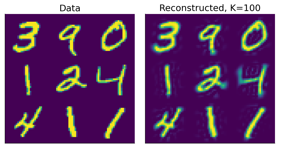
This is a great question. The main answer is that when X is reconstructed it should have the same number of columns as it did initially. Imagine the MNIST dataset which is a set of 28 x 28 pixels and 70000 photos. We don’t want the reconstruction to suddenly have fewer pixels! Just that some of the extraneous variance in the pixels be removed. So if we started with 70000 pictures by 28*28 = 784 pixels.
If we project it into component space we are now at 70000 by 784 components.
We could then take only the first 100 components now: 70000 x 100 components. We project these remaining components back using the corresponding eigenvectors[:, :100] transposed. Notice you also crop the eigenvectors but not in both dimensions.
70000 x 100 (projected data) @ 100 x 784 (cropped eigenvectors) = 70000 x 784 (back in pixel space now)
The cropped eigenvectors now translate those 100 components back to the original 784 pixels therefore removing the variance that was attributed by the discarded 684 components. And (to finally answer your question) this means we have to add the X_mean vector, in its entirety, back to the reconstruction. Because all pixels remains in tact.
Hope that helps!
1 Like
So if i’m getting it right, eventually in the reconstructed matrix the 684 truncated features columns would simply be composed by the mean of each of these columns for every row?
Thanks!
You’re right that 684 components have been truncated in the projected space. In feature (or pixel) space, those 684 components explained variance in all of the pixels. You reduce variance across all pixels but you don’t zero out any particular pixels. Let’s go back to the picture:
Each pixel in the image is a feature here. The way you have described it, 684 individual pixels (85% of all pixels) would be dead (like on a broken monitor). But this is not what has happened. There is still some variance in all (most?) pixels (… not sure about the edges) but the variance per pixel has been reduced by removing these 684 components.
All features remain and are unlikely to be (or at least, not necessarily) zeroed out entirely by PCA dimensionality reduction.
You say we “remove” these 684 components but that we are not zeroing the variance in those columns. So I don’t understand what we actually do to those features? just further reducing but not zeroing the variance in them? by what sort?
Thanks for the patience
I think it is a confusion between projected space and feature space. You start with your pixels in “feature” or “pixel” space. Each column is a pixel. Then you run PCA and your data is projected into a new set of basis vectors. This is now in “projected”/“component” space. Now your columns are each a component in projected space. Each column is NOT a pixel after the projection. It is a “component” which is organized along the directions of greatest variance.
You can “remove” these components by zeroing them out exactly as you say. But again these are components and not pixels. You can than project your data back into pixel or feature space. Now each column is again a pixel. And there should be data in each pixel. The effect of removing components (back when we were in projected space) was to reduce the variance in each pixel but it doesn’t explicitly zero-out any pixels at all.
So we zeroed the variance in 684 features as they are in the PCA components space, which are not original pixels but compositions of original pixels. Then we reconstruct the “surviving” features back to the original dimensions where they represent the pixels and we add each pixel its original mean.
BOOM! Exactly. That’s a better explanation. Thanks for that
1 Like