Let’s use this topic as Q/A for W2D1-W2D5
Happy learning!
Let’s use this topic as Q/A for W2D1-W2D5
Happy learning!
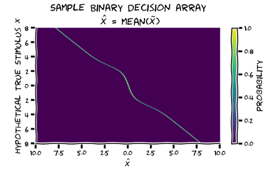
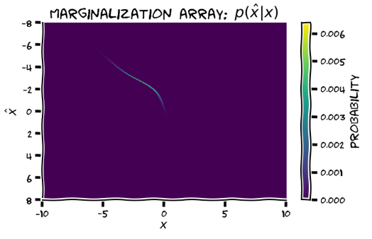
W2D1, Tutorial 3, Exercise 6:
Are the axis labels for the marginalisation array swapped?? Unless I’m missing something, these can’t be both correct:
W2D1 T1
In the text above exercise 2B, it is asked to compute the mean of the posterior distribution. I think there might be a x missing in the continous form :
Without this x, the integral gives 1 since we are integrating the pdf over its domain.
Question about W2D1_T3: I am confused by the mathematical notations here. How is the equation in Video 6: p(x_hat | x) = integration( p(x_tilde | x) f(x_tilde) dx_tilde) related to the illustration and explanation in Introduction (between Video 1 and Section 1)?
For exercise 1 of W2D1, the solution has px = np.exp(- 1/2/sigma**2 * (mu - x_points) ** 2), which is subsequently normalized. Why does the solution leave out the coefficient 1/sqrt(2pivariance) shown in the general form for the Gaussian?
I find that exercises in tutorial 3 are presented and solved in a confusing and inconsistent way.
There are three variables of interest: x, x_tilde, x_hat.
Here’s what I find confusing or misleading:
So far we’re computing the way the subject generates the response.
Next the marginalisation should be so that we can get p(x_hat|x), which depends on the parameters of subject’s priors, so that we can then infer these. So marginalisation should happen over x_tilde, but I’m very confused as to how exactly that’s implemented.
whether you leave the 1/sqrt(2pivar) out or not in this case is the same, since it will dissappear when you normalize: it will appear in each entry of px, and therefore also in the np.sum(px), so it gets cancelled in the normalization.
I agree… so far my head have been jumping between “ok i think i understand it now” and “wait it doesn’t seem to be what I thought”…
This question was posted to Slack and has been forwarded to content creators, but I wanted to repost here to keep q’s about W2D1 all in the same place.
Question about W2D1_T3 Ex. 6: Should we be summing “marginalization_array” over axis=1, not axis=0, and thus summing over x? If correct, this would also require changing 1st input when plotting “marginal”. If that’s wrong, could someone explain why p(x_hat) should peak close to 0, as shown in the output for Ex. 6? Thanks
Regarding W2D1T3, in the video and explanations, it seems like the matrix should have each row representing encoding position (x_tilde) and each column representing the stimulus location (X), but it is flipped for most of the matrices we built with the code.
Furthermore, the flip doesn’t seem to be consistently correct. Such as for the prior matrix, since the notebook is using “hypothetical true position” as X. then, the high probability stripe should probably be horizontal instead of vertical, if we are using the flipped labels.
Also second some of the questions @elena_zamfir mentioned.
:)) yes, there doesn’t seem to be a consistent way to imbue it with meaning… 
Not sure if this is helpful since I am as confused as you are, but I feel for the last point that you mentioned (changing from x_tilde to x_hat) is probably because we are estimating the optimal participants response (x_hat) from their brain encoding (x_tilde). Therefore, after we take the optimization (take the mean here), the x_tilde become x_hat, which is our estimate of participants response.
So the coefficient would be necessary if we were instead integrating the Gaussian from -inf to inf, but in this case it is not, because we normalize manually. Got it. I thought this was the case, but wanted to be sure in case my students take a look at the solutions and wonder why it was left out. Thanks!
that’s indeed what we are doing, setting x_hat as the mean of the posterior p(x|x_tilde), but then the variables in the matrix should be x_tilde and x_hat. indeed p(x_hat|x_tilde) has all the weight on one entry, the mean of p(x|x_tilde). but we haven’t yet computed p(x_hat|x)
exactly, the stripe should be horizontal for the prior, if we’re consistent, and given the way matrixes are multiplied to get the posterior
actually… you can use the coefficient term for normalisation, but you need to *dt as well. And I think that’s the “proper” way of normalising the Gaussian, as in the solution he said /sum() is proper only if we include similar number of points on both sides of mu.
Thanks! Yes, that makes perfect sense. I had noticed before that pre- and post-normalization, the curve was scaled by a factor of 0.1. Now I realize that this is just the dt that was used in the arange function.
W2D1 tutorial 3, section 5 onwards:
can someone explain conceptually why we need to further apply a gaussian over the true stimulus on each given trial? Do we think of this just as noise in the stimulus itself?
Yes! Nice catch. Will try to push out a patch for this shortly.
I think you are right and the ax-labels need to be swapped in the second one
MANAGED BY INCF