Bayesian W2D1 Tutorial 1

[Sunidhi]

When does the prior have the strongest influence over the posterior? When is it the weakest? What exactly are the answers of these questions asked within the tutorial after exercise 2A?

[aplumley]

From my understanding, the influence of the prior is strongest when the sigma of the likelihood is large. That is to say that the measured information provided has high uncertainty. In those cases, the posterior distribution mostly resembles the prior (our expectations), since the measurements are so uncertain/noisy that they have negligible effect on the posterior.

Conversely, when sigma of the likelihood function is small (we are very certain about the measured information), the prior has less influence.

[roschkoenig]

Exactly - if you play around a bit with the widget, you should be able to see a couple of the following observations

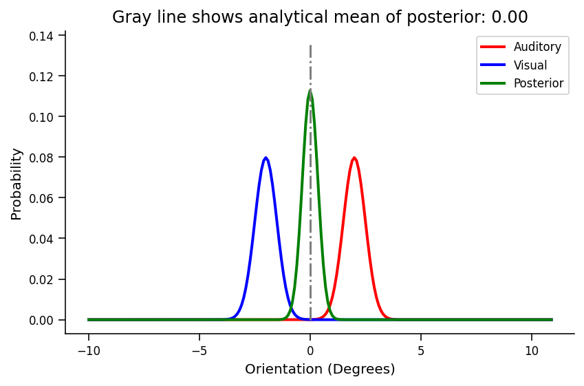
• if the sigmas of prior (visual) and likelihood (auditory) are equal, the posterior distribution is exactly in the middle
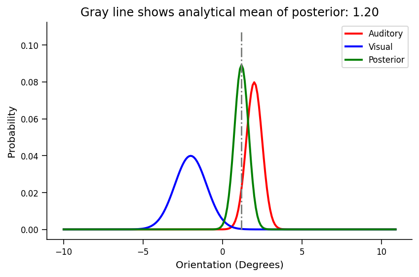
• if the sigma of prior is bigger than that of likelihood, the posterior distribution is closer to the likelihood
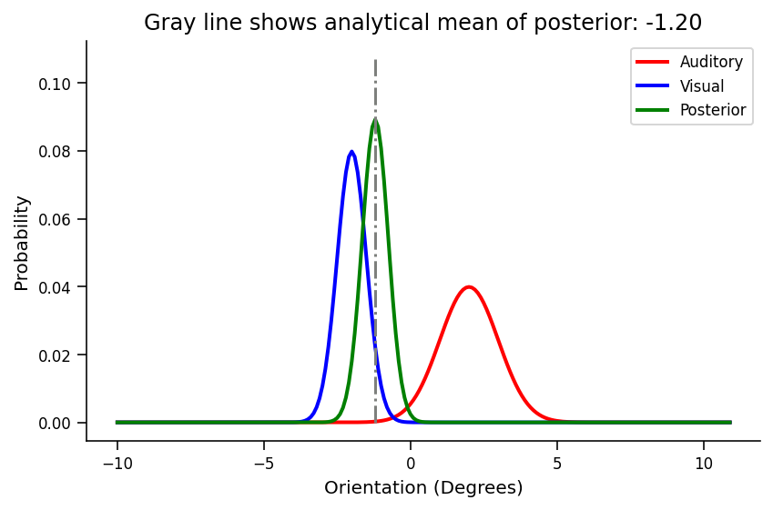
• conversely, if the sigma of the prior is smaller than that of the likelihood, the posterior distribution is closer to the prior

The overall take-away here is that probability distributions (likelihood, or prior) that are 'narrow (i.e. encode a certain variable with little uncertainty) have a big impact on the posterior distribution

[roschkoenig]

Some examples below

Below prior and likelihood variances are the same (sigma_auditory = sigma_visual = 0.5)

Below, prior variance is bigger (sigma_visual = 1.0) than likelihood variance (sigma_auditory = 0.5) and the posterior is much closer to the auditory distribution.

And lastly, the prior variance here is smaller (sigma_visual = 0.5) than the likelihood variance (sigma_auditory = 1.0) which results in the posterior sitting much closer to the prior

[mrkrause]

That’s a great answer!

Bayesian methods are often used to characterize beliefs, and thinking about it that way can be a good way to develop some intuition. The prior captures your…prior beliefs. The likelihood provides some sensory evidence, which you merge into the prior to produce the posterior. (Prior means before, Posterior=behind (or after) seeing the evidence).

For the localization example, we can think of the mean µ as “what we believe” and σ as inversely proportional to how sure we are in that belief. (In fact, some people use τ = 1/σ² instead, which they call “precision”, but let’s not dive down that particular rabbit hole just yet). A distribution like N(0,5) therefore suggests that you think the location is somewhere around 0, but you haven’t located it precisely. Something like N(5,0.01) means you’re very sure it’s located at 5.

So…when should your beliefs (=posterior) change a lot? Well, if you start with vague suspicion that something is true (=large sigma on prior) and someone gives you strong evidence that it is (narrow sigma for likelihood), your resulting belief should be strengthened (=posterior with narrow sigma). On the other hand, if you believe something strongly (=narrow prior) and someone presents you with unconvincing evidence (=broad likelihood), it shouldn’t change your beliefs much, and so the posterior doesn’t change. Finally, suppose you are moderately convinced that the stimulus is at µ1, but see some equally convincing evidence (i.e., the same sigma) that it’s actually at µ2. The rational thing to do would be to assume that both of your measurements are a bit imprecise, and it’s actually in the middle.

In all three cases, that’s how the math works out!

[aishling.cooke]

In our group, we were wondering why in Section 1/Exercise 1, the example code implemented a different formula to the Gaussian formula given directly above (specifically, it lacked the constant term) - is it just because that term is irrelevant when you normalise?

[aducote]

Yes. The coefficient would serve to normalize that posterior if you were integrating from -inf to +inf. However, in this case, we are only looking at a certain range and are integrating by summation rather than analytically. If you include the coefficient and don’t normalize, you might notice that the posterior curve is too large by a factor of 0.1. This 0.1 just happens to be the dx separating x’s in the original distribution. If you multiply that in when you calculate the posterior, the normalization is again done automatically.