Hi there, I’m a master’s student working on a project where I would be interested in using DCMs for the analysis of EEG data I have. Specifically using DCMs for Cross Spectral Densities since the data is resting state.
I figured going through the associated tutorial in the SPM12 documentation ( 1 ) would be a good place to start. However, I’m not able to reproduce the plots for the trial-specific effects and Bayesian Model Selection section.
Looking at the plots produced after model inversion it’s clear that the model doesn’t
fit well the data (cf. section 1). I’ve also tried running the DCM inversion as a script (cf. section 2).
If anyone is familiar with DCMs for EEG it would be very much appreciated if they could share feedback if parts are missing in the script I provided and if they too have encountered difficulties reproducing this tutorial. I was also wondering if there are hyperparameters that can be adjusted for the optimization process of the negative free energy done during model inversion. I’ve searched through the SPM12 manual but couldn’t find anything.
Many thanks in advance!
As a side note, I get the same results as the tutorial with DCMs for evoked responses.
1. Plots reflecting poor fit of the model and different results than the tutorial :
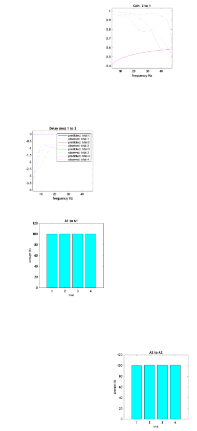
No screenshots are provided in the tutorial for the fit of the DCM but mine is really poor (so there is no real reason to believe that the rest of the results will be sensible). The model converged after 20 or so iterations of EM for both models being tested (with intrinsic or extrinsic connections being modulated).
Ab love is an example for the coherence of channels where there is a clear discrepancy between the predicted and observed traces.
Below are the trial-specific effects I get (barely any modulation)
2. SPM Batch
Considering the possibility that the issue had something to do with the GUI I wrote the steps as a script but the same results were yielded.
DCM=[];
DCM.name        = 'test_CSD_DCM';
DCM.xY.Dfile    = '/MyPath/DCM_CSD_tuto/dLFP_white_noise_r24_anaes/dLFP_white_noise_r24_anaes.mat';

DCM.Sname       = {'A1';'A2'};

% same as what was produced for the CSD LFP tutorial
DCM.xY.modality = 'LFP';
DCM.xY.Ic       = 1:2;

DCM.options.Fdcm    = [4 48];
DCM.options.trials  = [1 2 3 4];
DCM.options.Tdcm    = [250000 30000];
DCM.options.D       = 1;
DCM.options.spatial = 'LFP';
DCM.options.analysis = 'CSD';
DCM.options.model = 'CMC';
% QEST: why wasn't the analysis type specified in the example script?

DCM.A{1}        = zeros(2,2);
DCM.A{1}(2,1)   = 1;                %A1 -> A2 modeled as forward connection

DCM.A{2}        = zeros(2,2);
DCM.A{2}(1,2)   = 1;                %A2 -> A1 modeled as backward connection

DCM.A{3}        = zeros(2,2);

DCM.B{1}        = zeros(2,2);
DCM.B{1}(1,2)   = 1;                % Model 1: extrinsic connections (off-diagonal entries) are modulated
DCM.B{1}(2,1)   = 1;
DCM.B{2}        = zeros(2,2);
DCM.B{2}(1,2)   = 1;                % Model 1: extrinsic connections (off-diagonal entries) are modulated
DCM.B{2}(2,1)   = 1;
DCM.B{3}        = zeros(2,2);
DCM.B{3}(1,2)   = 1;                % Model 1: extrinsic connections (off-diagonal entries) are modulated
DCM.B{3}(2,1)   = 1;

DCM.xU.X        = [0 0 0; 1 0 0; 0 1 0; 0 0 1];           % REV
DCM.xU.name     = {"effect 1"; "effect 2"; "effect 3"};


% testing with DCM made with GUI
DCM_extr_CMC = load('/Users/abelrassat/Desktop/NSC/Computational_Phenomenology/DCM_CSD_tuto/DCM_extr_CMC.mat')

disp(DCM_extr_CMC.DCM.xY.Dfile)

DCM_extr_CMC = spm_dcm_csd(DCM_extr_CMC.DCM);
3. Versions:
I’m running SPM12 with Matlab 2018b on a Mac OS.