Hello tedana experts,
We are trying to set up a pipeline for our ME dataset (3 TEs and 203 TRs), and tedana identified few BOLD components (<10). I wonder if that might indicate an issue with our preprocessing or data. We are using fmriprep v22.0.1 with --me-output-echos (fmriprep seems to be working properly judging from the T2* map and histogram). The preprocessed ME data (*echo-x_desc-preproc_bold.nii.gz) were then passed onto tedana 0.0.12 with all default settings. I also tried with different tedana settings but got very few accepted components.
Looks like about 30 components from 203 timepoints - that is lower than I would expect. I have some questions that might get us pointed in the right direction.
Can you provide the details about the sequence, such as coverage, TR, voxel resolution, Multiband, GRAPPA/SENSE, TEs, field strenght, number of channels in head coil and all of those fun things? Was this a task or resting state?
Was slice timing performed?
If you inspect the combined timeseries, does it look reasonable - as in, does it seem like motion correction worked, etc?
What other settings did you try? A more liberal PCA selection method (aic instead of mdl) or even the alternative kundu approach?
How do the rejected components look, does it seem like mistakes were made? In other words does it looks like it rejected things that fit a task (if performed) or typical resting state networks, or does it seem like it did an ok job?
Do you just have one example dataset or are you seeing this strange behavior across multiple participants?
I agree with @dowdlelt that the total number of components (32) seems a bit low. In general, PCA fully models the data, but we don’t want PCA components that are essentially Gaussian (thermal) noise. Therefore, there are a bunch of methods that can be used to estimate the amount of Gaussian noise in the dataset and then only retain the number of components that structured signal.Those components are what are used for ICA and then multi-echo component selection.
Unfortunately, while we’re using a widely accepted method to estimate the number of PCA components, we’re also seeing more and more cases, like this, where the estimate is way too large or small. As @dowdlelt mentioned, there are a few different criterion methods to identify the cut-off. We changed the default to AIC in version v0.0.12 and that should already give you more components than the other built-in options. I am working on better methods to calculate the total number of components.
For now, it would be useful to confirm this is what’s happening. There are two ways to do this. First, if you’re running tedana on multiple datasets and the total number of components normally seems reasonable, but is too low/high in a subset that’s a sign that this is the issue.
Last May we also added these PCA fitting curves as default outputs. We haven’t created a new version since then so you’d need to download the code from the github repo and install. You then get image like on the top right of our OHBM 2022 poster that could help me better understand the issue.
The post v0.0.12 also allows users to enter a hard-coded number of components or the expected variance explained for the components. This isn’t an ideal solution, but, if most of your data seem fine and there are a few weird runs, this might be a hacky, but reasonable way to address the problem.
Can you provide the details about the sequence, such as coverage, TR, voxel resolution, Multiband, GRAPPA/SENSE, TEs, field strenght, number of channels in head coil and all of those fun things? Was this a task or resting state?
From the GE protocol, it appears to be 3T, 3mm isotropic voxel, single-band EPI, TE=12/24.5/36ms, 32-channel head coil. Also a task data.
Was slice timing performed?
Yes.
What other settings did you try? A more liberal PCA selection method (aic instead of mdl) or even the alternative kundu approach?
I tried forcing more components=100 and results remained similar (few accepted components), and I will try aic.
If you inspect the combined timeseries, does it look reasonable - as in, does it seem like motion correction worked, etc?
Well, I am not too worried whether it removes motion, but rather whether it removes too much variance from the data (throwing the baby out with the bathwater) given the #rejected vs #accepeted. To answer your question, the denoised data seems to be smoother than the original data (less spiky) and I would think tedana did a good job removing motion artifacts.
How do the rejected components look, does it seem like mistakes were made? In other words does it looks like it rejected things that fit a task (if performed) or typical resting state networks, or does it seem like it did an ok job?
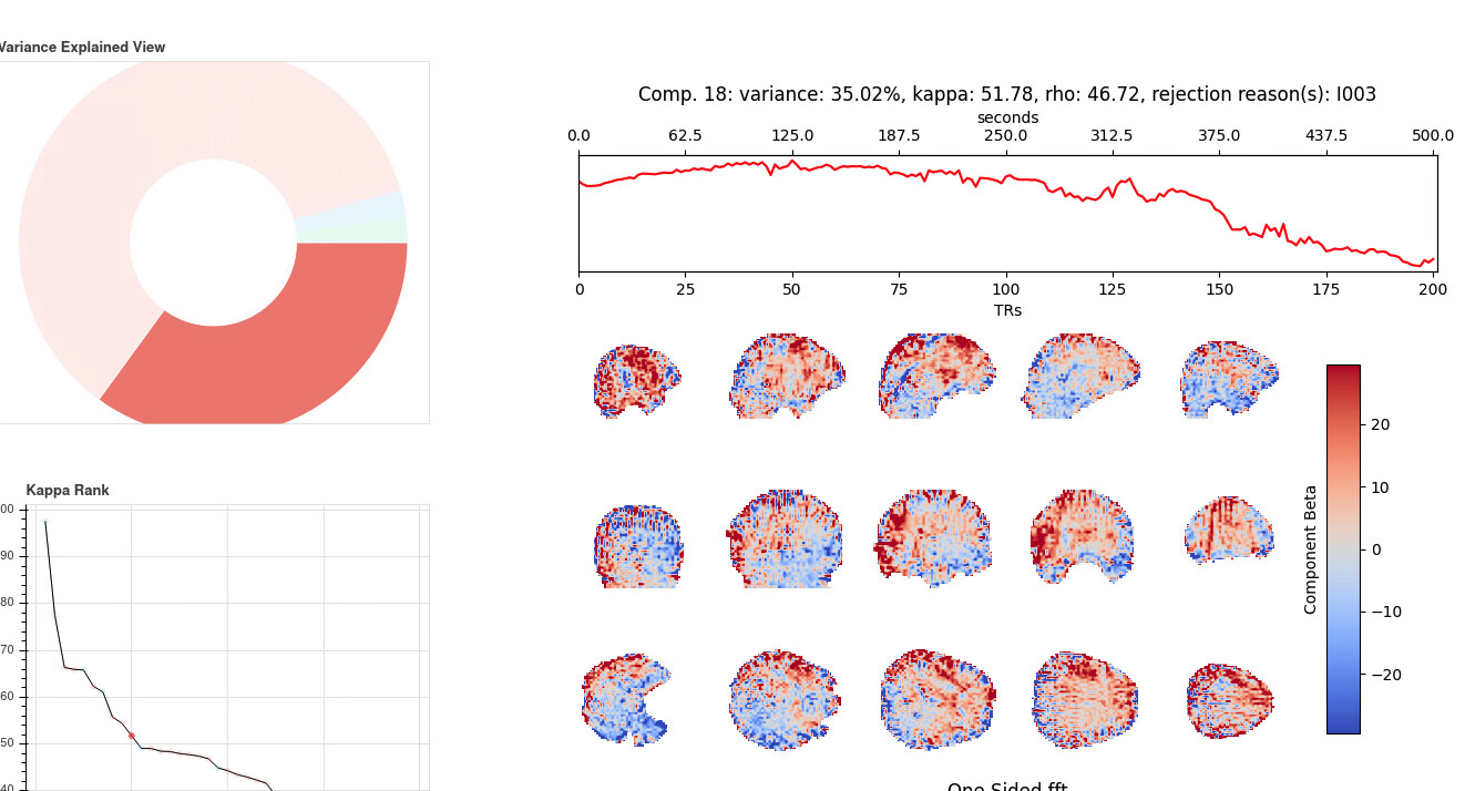
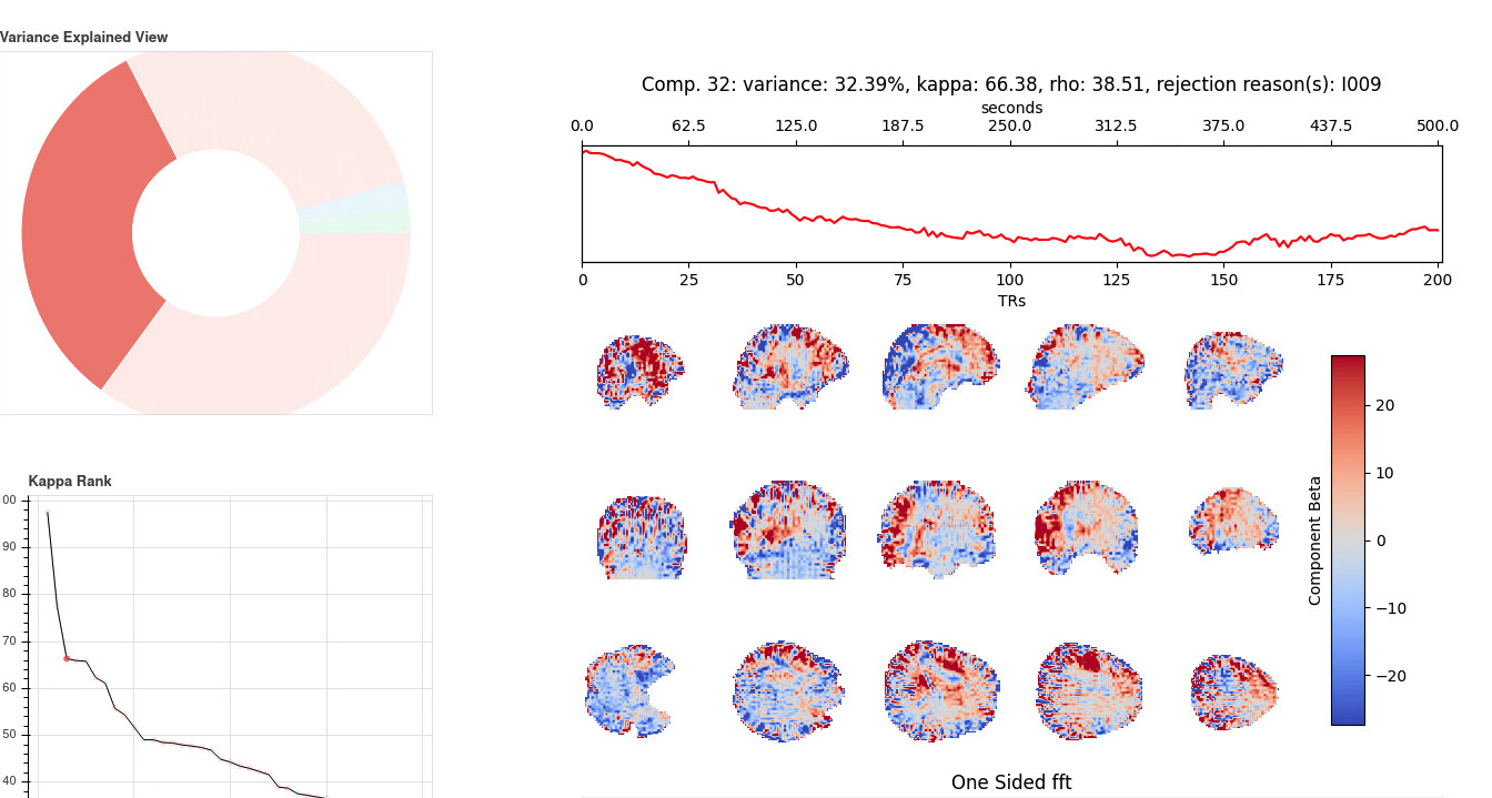
I am not familiar with tedana ICA decomposition but it does not appear any of them resemble the RSNs. But the two rejected ICs with a lot of variance appear to reflect some kind of scanner drift (or global trend), but is this something that I should be concerned?
Do you just have one example dataset or are you seeing this strange behavior across multiple participants?
I only have one subject but will get more subjects very soon.
Thanks for the prompt answers. I think @handwerkerd suggestions are all worth following up on as well.
Since this is just one subject, I think it is too early to be certain or not if there is something wrong. A few clarifications on my questions.
Regarding motion - I was less concerned with tedana removing motion and more asking if the preprocessing from fmriprep was successful. I have no reason to think fmriprep wouldn’t work well, but if something went wrong there, then there isn’t anything tedana could do to help. Given that you have fairly standard data, I imaging that went fine, but it may still be worth watching a movie of the data, inspecting the motion parameters and such just to make sure this isn’t a ‘garbage in, garbage out’ problem.
Regarding the point of throwing out too much signal, that is an extremely valid concern - and the best I can suggest there is to look through all of the components to make sure nothing looks (in the time course sense) like your task paradigm or looks like something like a contrast map - for example, if I was doing a visual task and there was a component that looked like visual cortex activation - that might (or might not!) be an issue. Just a general inspection of all of the components can be useful, though I understand not all tasks are so easy to visualize in timecourses.
For the components you highlighted, that isn’t a problem at all. The timecourses do look like slow movement or scanner drift over the course of the acquisition. Those being removed is a good thing. That said, the structure that is visible in those is a little odd, so I would want to look at the data itself to make sure there was no strange artifact in the acquisition, like aliasing or ghosting. I’m specifically curious about the vertical stripe like bits in the most anterior coronal section, and the ring-like alternating red/blue patterns in the axial sections - anything like that in the raw data that is visible to the eye?
Also - is this something where you can look at the single subject statistics and compare before and after denoising to see if things worked well?
Hi Dan,
Thank you! This is very helpful. I will try different tedana configurations and verify with more datasets to see if this is reproducible. Also while playing around with tedana final denoised output using FSL, I observed a much higher correlation between any given seeds and the rest of the brain than prior-tedana. I wonder if that is what you would expect from tedana. Another question is that if you compare single-echo GLM results with multi-echo ones (like in this paper, would you expect tedana denoised data to have more expansive activation pattern?
Thanks,
Oliver
I’m realizing one key confusion you might have. “Ignored” components ARE retained in the denoised time series. This is a legacy terminology for several component classification criteria for borderline components. The idea was, if a component wasn’t definitively T2* but was either too low variance to bother with or some mix of low variance and some T2* signal, then don’t call it T2* but also don’t remove it. I think this is why you data looks ok even if there seem to be few accepted components.
I really don’t like this terminology because it is confusing. For a major change to the code that is very close to done this terminology will be changed. Everything that is retained will be classified as “accepted” but there will also be tags to better understand why specific components were accepted.
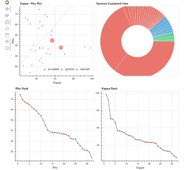
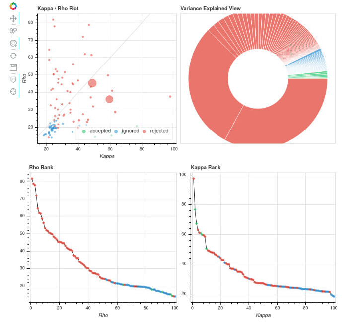
Looking at your kappa vs rho scatter plots, your original one looks ok. For the one with 100 components, you can see a bunch of components with very high kappa that were rejected. Those are the ones I’d look at most carefully. For example, there’s one with kappa>95 and rho<40. I’d assume that might contain some S0 signal, but I suspect there’s enough T2* signal that it shouldn’t be flat out rejected.
For single vs multi-echo GLMs, I’d expect an increased contrast-to-noise ratio in most participants (0-30%, avg 8% in one of my datasets) . That would mean voxels that might be slightly below threshold with single echo would be above threshold with multi-echo. FWIW, I’m not fond of the figure 1 in the linked paper because, if you regress out signal with ICA or any other method, TSNR (mean/variance) will increase. It’s not particularly interesting to say “If I remove variance TSNR goes up” That’s why I try to focus on areas of expected activity and compare contrast-to-noise for expected responses.
Ignored” components ARE retained in the denoised time series.
Thanks, Dan. That makes so much more sense now. Would definitely be helpful to have more consistent terminology with either accepted or rejected.
For single vs multi-echo GLMs, I’d expect an increased contrast-to-noise ratio in most participants (0-30%, avg 8% in one of my datasets)
This is good to know. I wonder what nuisance regressors would you recommend including the GLM analysis? Same as single-echo? ICA-aroma recommends WM and CSF instead of motion parameters.
I’d think about additional regressors the same as you would for single echo. I tend to include motion and first derivative and not CSF & WM for task studies. CSF should be fairly well covered by multi-echo denoising and I’d be hesitant regarding whether the WM ROI ends up with some task-locked signal that you don’t want to remove. I’m sure others could hold different but perfectly reasonable positions. My general approach is to look at how noise regressors fit the brain. For example, if the WM fit looks a bit too much like a gray matter task response, that’s a warning sign.