Hi all,
I’m having difficulty trying to plot an atlas as well as a statistical map onto the same cortical surface with nilearn.
I want to plot the Yeo functional atlas onto the cortical surface, and then overlay it with my cluster results. I can plot them separately, but I want to overlay them on 1 brain.
Does anyone have ideas about how to do this?
My code:
from nilearn import plotting, datasets, surface,
#load my own data
map1 = ‘my_clusters.nii.gz’
mask1 = surface.vol_to_surf(map1, fsaverage[‘pial_right’],
inner_mesh=fsaverage[‘white_right’]) plot my own data - using figure=fig to plot over the atlas plot maps
plotting.plot_surf_stat_map(fsaverage.pial_right, stat_map=mask1, hemi=‘right’,
threshold=0.5,
alpha=0.1,
figure=fig,
)
plotting.show()
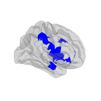
The output only shows my cluster:
I’m not sure if it supports fsaverage space, if not, you might need to re-run your analysis with Yeo’s atlas under HCP fsLR surface space (which is available in yeo’s lab github repo). If your data is of small amount it can be one way to try
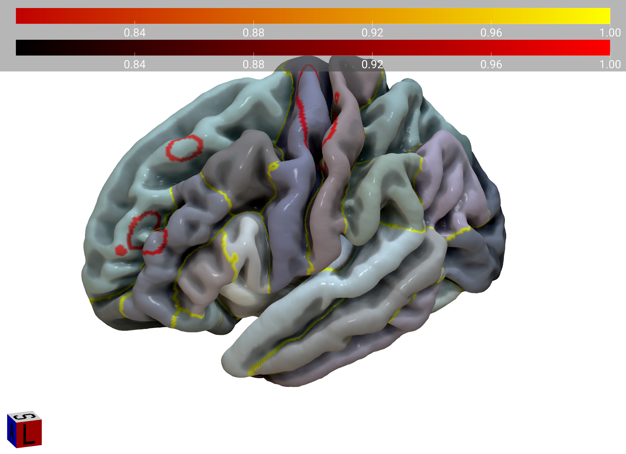
You might also consider Surfice. The image below is from Scripting/Templates/Outline, but you can remove the outline effect if you wish. The Surfice Python script is
import gl
gl.resetdefaults()
gl.meshload('lh.pial')
gl.overlayload('boggle.lh.annot')
#make contour at border of atlas
gl.contour(0)
#reduce atlas salience:
gl.atlassaturationalpha(0.2, 0.5)
gl.overlayload('motor_4t95vol.nii.gz')
gl.overlayminmax(gl.overlaycount(),-2,-3)
#hide statistical map:
gl.overlayopacity(gl.overlaycount(),0)
#draw outline of statistical threshold
gl.contour(gl.overlaycount())
When calling the “plot_surf_stat_map” function a new figure is created by default see plot_surf_stat_map documentation .
You can override this by specifying the same figure in plot_surf_roi and in plot_surf_stat_map (adding figure = f or something similar).
Thanks Haya! That’s why I specified 'figure = ’ for plot_surf_roi and ‘figure = fig’ in the plot_surf_stat_map command. Even when I include ‘figure = fig’ within the plot_surf_roi command it doesn’t work.
Sorry did not see it in the last call line… Have you tried specifying the same “axes” instead of figure? (maybe defining a figure before calling both functions something like fig, axes = plt.subplots(nrows=1, ncols=1, figsize=(10,10), dpi=400) then using the same axes in both plotting functions).
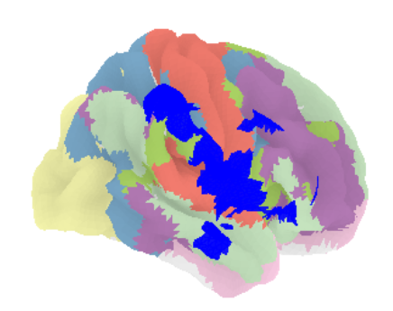
Success! Thanks so much @haya for your suggestions. Looking at the issue here, I needed to define the axis and then specify the surface subplot kwarg:
fig, axes = plt.subplots(nrows=1, ncols=1, subplot_kw={“projection”: “3d”})
My code:
from nilearn import datasets, plotting, surface
import matplotlib.pyplot as plt