I only ran slice-scan time correction and a six parameter rigid body motion correction (with the first volume of the run as the reference volume). The motion parameters are estimated based on the TE1 data and then applied to the other TE data. That should be it…
just as an add-on:
I had a closer look at slices 1/33/65 from volumes 1 and 172 of the TE1 dataset (acquired at 0/975/1947.5 ms into the TR respectively).
There’s a ‘zero intensity’ line at the edge of each image (also present in the original dcm to separate the slices) which adds up to ~1% of pixels in each slice. The performed preprocessing adds no additional zero-valued pixels for the ‘volume 1’ slices, and only increases the number of zero-valued pixels by <=1% for the slices in volume 172 (which should be the most strongly affected as volume 1 was used as the reference for the motion correction). In addition, most of these zero-valued pixels are located at the edge of the image (i.e., quite far from the brain data).
Furthermore, I also realized that due to the specified mask, none of the identified zero-valued voxels mentioned above should actually be considered when running tedana.
So in short, it looks like the performed preprocessing did not lead to any unforeseen outcomes, and even if it did, the provided mask should have prevented these voxels from being included in the first place.
Hopefully this information is still helpful. Please let me know if there’s anything else I could do.
Another update from my side:
I’ve cleaned up the nifti export (so the header information should be fine now) and re-ran tedana (both v0.0.9 and the latest v0.0.10 with a slightly more liberal mask):
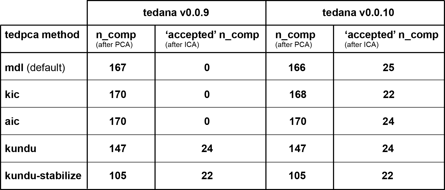
Interestingly, the v0.0.10 results show a rather consistent selection of ICA components. Moreover, the beta map of the component whose time series most clearly reflects the ongoing task now nicely shows the structure one might expect (whereas the corresponding v0.0.09 map doesn’t appear to show any particular spatial configuration).
Contrastingly, the somewhat surprising PCA results remain unaltered.
Did you perhaps have the chance to look into this issue further @jbteves / @e.urunuela ?
Thanks again for any input on this!
1 Like
Hey @exumbra ,
I just ran tedana on your data after some minimal preprocessing: I took the preprocessed data @jbteves shared with me, and did a 3mm smoothing, 6 order polynomial regression, and transformed the data into percentage signal change. I computed the mask with AFNI’s 3dAutomask function on the second echo data.
I got 72 components using the default tedpca option, i.e., maPCA with the MDL approach. I used the main branch which should be fairly similar in terms of performance to v0.0.10.
However, after seeing that the component maps were mainly blank, I saw that the optimally combined data used for maPCA was not correct. It looked nothing like fMRI data. Did the optimally combined data look good on your end @jbteves ?
First of all, thanks @e.urunuela for looking into this further and apologies for the delay in getting back into the conversation.
Did you by any chance still have contact with @jbteves related to your previous post? I was also wondering about the preprocessing you performed, as the ‘readthedocs’ currently state any pre-tedana preprocessing should be limited to slice scan time and motion correction. Are these recommendations still in flux?
As an update from my side, I’ve been looking into tedana v0.0.11 and the default ‘mdl’ resulted in 94-99% of components being kept after PCA across 4 runs in one dataset, and 91-99% in another dataset (with the exception of a single run in which only 30% of components were kept, appearing too aggressive). As a reference, when using 95% explained variance as a criterion, this led to 66-76% and 79-81% of components being kept after PCA for the same datasets, respectively.
So far, I haven’t been able to figure out what’s going on, but at least the latter results based on ‘variance explained’ look pretty consistent.
Thanks again for thinking along and your continued efforts!
Hi all, unfortunately this completely slipped my mind last May. @exumbra, I don’t have whatever I did anymore (I periodically cull my short-term data storage), but most likely I ran something like this:
afni_proc.py \
-blocks tshift volreg \
-subj_id ID \
-dsets_me_run DATA \
-reg_echo 2 \
-execute
Which would only perform slice-time correction and volume registration (motion correction).
@e.urunuela I don’t recall taking a very close look at the outputs, if you still happen to have the preprocessed data I’ll take a look.
Hi @exumbra ,
First of all, our recommendations on the docs have not changes.
I do not have the preprocessed data, but would gladly re-run the whole thing and try to look deeper into it if you send me the data.
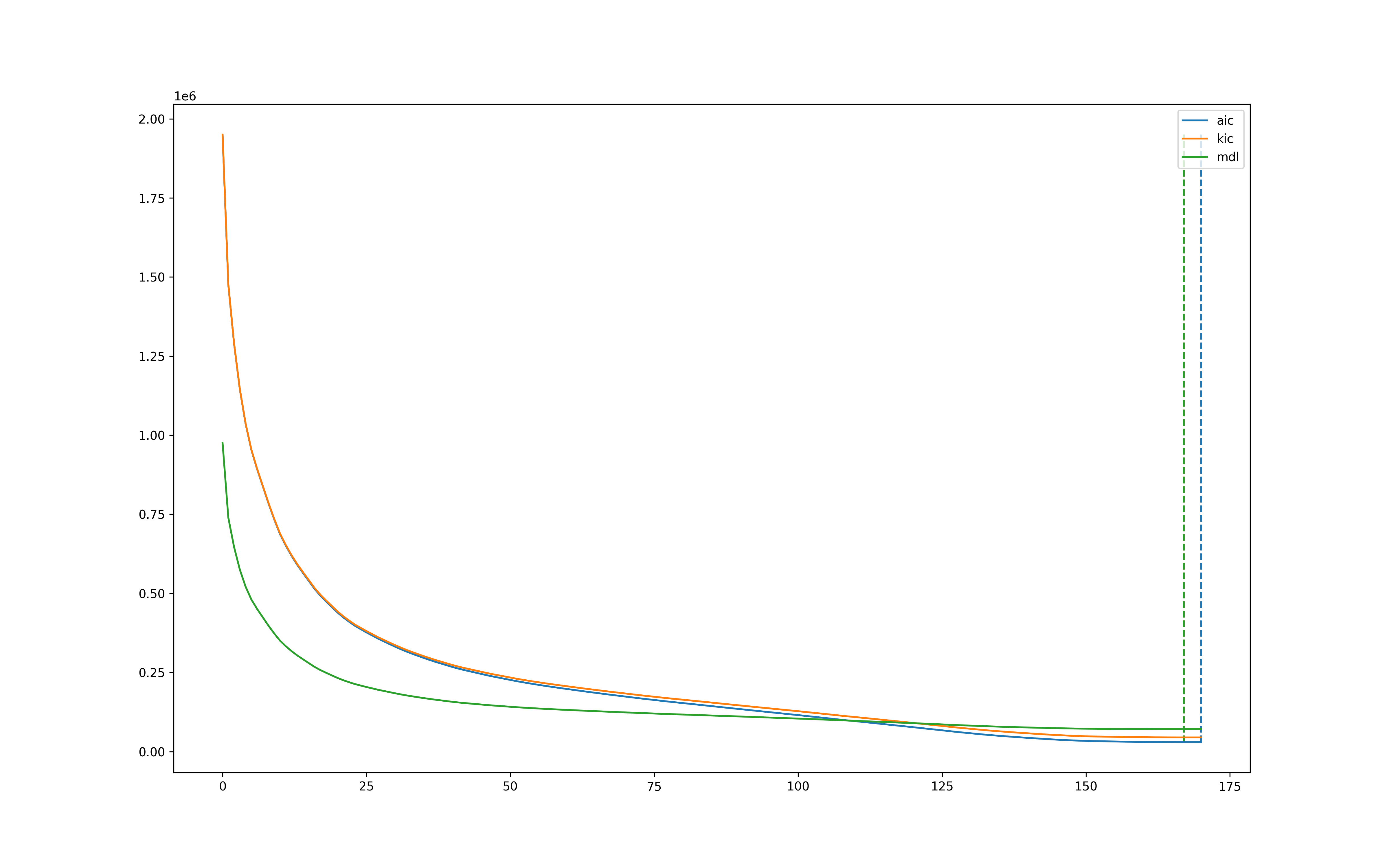
It is odd (but not impossible) that maPCA keeps a high percentage of components. This can happen if the optimization curve is rather flat, hence making it difficult to find the “elbow”.
We are currently working on making the different PCA options more transparent to users by providing the optimal number of components calculated by maPCA, along with some plots that should make it easier to follow the intuitions behind the method.
I would like to ask you to send the data back again so I can have a deeper look.
Thanks!
Thanks @e.urunuela @jbteves for your replies and your willingness to have another look.
I’ve send you a link with the dicoms just now…
Hi exumbra, do you happen to have another way to anonymize these files? I didn’t notice last time (… somehow… because it is very obvious now…) but apparently the matlab dicom anonymization you ran stripped some information out. See dcm2niix warning:
“Warning: Matlab DICOMANON can scramble SeriesInstanceUID (0020,000e) and remove crucial data (see issue 383).”
The linked issue is here: https://github.com/rordenlab/dcm2niix/issues/383
As you can see this makes it difficult to reconstruct a nifti file from the dicoms, and consequently any weirdness we see may be due to missing information. So to narrow things down, I’d prefer another batch of dicoms anonymized a different way.
thanks @jbteves for the pointer. I’ve uploaded another version just now and sent you the corresponding link. Please note that all of the observations above from my side could not have been affected by this though (as all of the steps were done pre-dicomanon).
Thanks for having another look!
@e.urunuela I’m taking a look at the data and if I just run normal afni proc with no smoothing and do standard motion correction with afni proc, then I get 172 PCA components (which is a lot, obviously) with mdl. The OC data does indeed look like normal BOLD data, just with a bit better contrast. However there’s a few interesting things:
- There are two components, rejected, that explain 74% (!!) of the variance. They’re very-slow-drift components, one of which seems to have magnitude increases (which then plateau) inversely correlated with some motion spikes.
- @exumbra is it fair to say that you have a block design that lasts about 25-30 seconds? If so you have a very strong accepted bold component that survives despite the weirdness.
- The component maps don’t look like they’re blank, they’re just for some reason not rendering in the HTML report. That said, many components basically look like a random voxel cluster experiencing very un-compelling white noise.
Thanks for having a look!
Regarding the points you mentioned:
- indeed, slow drifts can cover anything between ~15 to 72% explained variance (the run you had a look at is the most extreme example so far). That said, also for the run in which the explained variance for the slow drifts adds up to ~15%, the nr of kept components with ‘mdl’ is 90%, suggesting they are not the main contributors to the observed PCA issue.
- yes, every run I’ve looked at so far contains an accepted bold component which nicely seems to follow the task protocol.
- I haven’t seen any blank component maps either and ‘un-compelling’ does sometimes cover their content ;).
I have no idea what I did back in May 2021, but it looks like it’s all good on your end.
Most importantly, how many accepted components did you get? IIRC this was the reason for opening this post.
I’m not sure what @jbteves observed, but in my hands the shared run leads to 26 accepted ICA components (16%) using the mdl default, while using a 95% variance explained threshold for PCA leads to 27 (i.e., 24%) accepted ICA components. The same applies to the other runs from this participant (16-17% accepted ICA components vs. 20-24% for mdl vs. varex PCA, respectively).
Are these numbers in line with what you generally see?
Regarding the initial reason to start this post: it looks as if whatever caused the observation that hardly any BOLD components were accepted initially, has been solved by moving to tedana v0.0.11 (perhaps aided by the tweaks to the nifti headers mentioned above). However, the additional observation that the default PCA option does not appear to lead to a substantial reduction in components currently remains (although switching to a variance explained threshold appears to be a viable option for now as it appears to lead to consistent findings overall).
@jbteves could you share the exact afni proc command you used? I’d like to replicate your results on my end. I think I’ll have some time to look at this today. Thanks!
Edit: actually, it might be easier if you could share the nifti files you used with tedana.

Hi @exumbra ,
I’ve had a look at your data and I think it looks good. The PCA step is not reducing much of the dimensionality for whatever characteristics the data may have (I honestly don’t know atm). So I would suggest you stick to the 95% of explained variance criterion with your analyses until we have a better solution. At the end of the day, this is also a valid criterion to select the number of components to retain.
We will soon make tedana output the number of components that would be selected with each maPCA option, together with a graph that shows where maPCA finds the optimal solution (similar to the image below). I am confident this can be released soon. However, on the data you shared, I do not expect to see a higher percentage of accepted components if dimensionality is further reduced. I have actually tested if there’s any gain on applying skull stripping, smoothing, detrending, and conversion to percent signal change, and I have only seen a reduced number of accepted components with the addition of each of these preprocessing steps (because dimensionality was reduced down to even 55 components with mdl when working with PSC data).
In any case, I would say that we should focus our efforts on improving the classification of ICA components, as I see this as the more critical of the two issues. We have been working on a customizable classification for 2 years now, and it will hopefully be out soon (@jbteves probably has an estimate of when).
I am sorry I cannot be more helpful at this moment.
Hi @e.urunuela ,
thanks so much for having a closer look! I’m happy to hear you think everything in principle looks OK and using the 95% explained variance option is a good way forward for now.
The added tedana output you mentioned certainly sounds helpful (could it also include a chosen varex threshold as reference perhaps ;)?) and I’ll keep an eye out for any future releases then!
I think it should be straightforward to add the varex info too. I’ll try to open a PR some time this week.