I have two clarification questions about using fmriprep (21.0.0) with tedana (0.0.11). My dataset is 3T resting-state with 1 run, 3 echoes that was pre-processed using fmriprep for head motion correction.
How does nilearn’s compute_epi_mask on the first echo compare to fmriprep’s mask for the bold images? That is, are the differences in inclusiveness in the initial mask (if any) appreciable after subsequent adaptive masking? I want to maximize coverage in areas that typically have low signal, which seems to have been largely addressed by the recent 1 vs. 3 echo thresholding change in tedana. Not sure if tweaking the initial mask will aid this goal much more. @tsalo I noticed your notebook on tedana used fmriprep’s bold mask as an explicit mask, which prompted the question.
My second question is about when you might consider dropping a subject from further analysis based on the # of accepted components and/or their variance. I have played around with the seed and tedpca options (mdl, kic, aic) to get a sense of the # of components and % variance of accepted components that are typical on my data. As an example (using mdl and a set seed), sub-0611 has comparatively similar # of accepted components accounting for little variance compared to, for instance, sub-0010 who is fairly typical of the dataset. I understand if folks are hesitant to say X # of components and/or X % of variance explained, but is it reasonable to think that I should drop 0611?
I believe there could be meaningful differences. compute_epi_mask is a lot simpler than fMRIPrep’s brain mask creation, and I think it’s meant more as a quick solution than a complete replacement for more complex mask creation methods. Unfortunately, I don’t know what effect the different approaches tend to have on the resulting brain masks, but I would use fMRIPrep’s as a general rule.
I think I should ping @handwerkerd on this one. We don’t have any recommendations about run-level quality control in our documentation, which is probably something we should address. My first thought, though, is that I would probably do what they recommend for MRIQC, which is to run the workflow on the full dataset and then look at the distribution of QC metrics across the dataset to identify outliers. In this case, you could use the variance explained by rejected components (since accepted and ignored components both end up in the denoised data) to see if there are runs with exceptionally large amounts of variance being removed.
I did some testing on a few subjects and it looks like fmriprep’s bold mask tends to result in a more inclusive adaptive mask (esp. in subcortex and OFC) than compute_epi_mask, if there are major differences. The component selection/classification changes too, with greater differences when the masks are more different. It’s only a few subjects but that would make sense to me as a potential tradeoff to consider.
Makes sense to use information about the full dataset. And yes, I’d love to hear other thoughts on what is good to look for on the run-level.
I agree that we should write more about run-level quality control in our documentation. In general, I’d say that the one thing I’d consider a serious warning sign is if the total variance explained by the PCA/ICA is very different in one subject vs others. This is in the tedana_[date].tsv file and it’s marked by “Variance explained by ICA decomposition: X%” (Second note-to-self: This should be presented in a more prominent location). That percentage will vary based on acquisition choices, but if acqusition are identical within a study (including run length), it should be fairly stable. If one run has a much lower variance explained, that’s a warning sign.
I’d similarly expect a roughly similar number of accepted components across runs, but there will be variation. In the above example, you have 4 accepted in one run and 6 in the other. These both seem a bit low to me (do these runs have less than 150 time points?) but that difference isn’t huge. I wouldn’t worry too much about relative variance explained between run because there are good reasons that can vary. For example, if one run has a larger linear drift or greater head motion, then you’d hope that a lot more variance explained ends up in a rejected component. I suspect that’s part of what’s happening with the two very high variance rejected components in sub-0611.
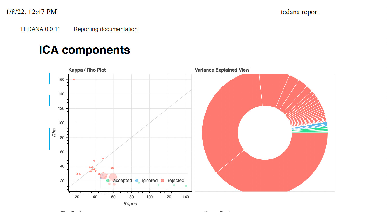
That said, any time things look a bit odd between runs, that’s a good excuse to look a bit more carefully at components on the report page. I guarantee that the current component classification method is not perfect (we’re working on it!) I suggest looking at the spatial maps and time series for the very high variance components to make sure they really look like linear drift or motion. Also look at the “rejected” or “ignored” components with the highest kappa values. If a rejected component in sub-0611 looks really similar to an accepted one in sub-0010, it may be worth manually accepting it.
Thanks for the detailed suggestions! I will take a look at what is typical across subjects and manually inspect high variance and high kappa ignored and rejected components. These responses answer my question about how to assess run quality.
For context, my question was motivated by my experience with MEICA v3.2 in AFNI where - in another rest dataset - we saw many more components overall, and generally took a closer look at runs with fewer than 10 accepted components. Even knowing the component selection/classification is different for a variety of reasons in tedana, the accepted components here seemed low.
My data has 200 older adults with 1 rest run per person. There are 604 time points (1s TR, so ~10 minutes), 3 echoes (12, 30.11, 48.22 ms), and multi-band acquisition. Across 15 test subjects (using default ‘mdl’ tedpca option, default compute_epi_mask), the average variance explained was 87% (80-94), total components was 31 (22-40), and accepted components was 7 (4-10). I saw previous forum/github posts about the wrong or corrupted files being submitted to tedana. But, the echo-specific outputs after head motion correction (no STC/SDC) using the new --me-output-echoes flag look fine to me.
I have datasets with 90-94% variance explained, but 87% variance explained is very reasonable.
For 604 time points, having 22-40 total components seems low to me. 22 is very low. For the same data do you know the typical number of components with MEICA? The other thing that would affect the total number of components would be the number of voxels in the brain. if your data include the majority of the cortex and are 3mm^3, then I’d still say this is surprisingly few components. This is also where an overly aggressive mask can cause a problem. If the other masking issues you mentioned removed too many voxels from the dataset, then that would also affect your total number of components.
Assuming your masking concern is now resolved and you’re still getting these low numbers of total components, you might want to use another option for the pca step. ‘mdl’ should be the most agressive and will give you the least total variance explained and the lowest total number of components. ‘kic’ is moderate, and ‘aic’ is more liberal. This isn’t a part of the code I developed but, perhaps @eurunuela can tell you why mdl is the default and if you should have any concerns using the other options.
There are differences in the PCA and component estimation step in MEICA vs tedana. MEICA did something “under-documented” but interesting. It calculated T2* & S0 estimates of the PCA components and used that that information to reject some PCA components. In our hands, this was sometimes very effective, but, in some datasets, this component rejection process seemed to cause problems in ways that were hard for an end-user to notice. We opted for a more generalized and standard method (https://github.com/ME-ICA/mapca) that we ported from GIFT.
FWIW, I think AFNI still ships with MEICA v2.5. MEICA v3.2 includes some cool ideas, but a lot of it wasn’t robustly validated across multipe types of data sets and the code was brittle. tedana is a fork of MEICA v2.5. At some point, it may be worth revisiting v3.2 to see if we can pull some of the ideas implemented there into tedana.
Gotcha - it’s helpful to hear what you’ve seen in other datasets. Yes, my data is 3mm^3 and most cortex. The numbers I reported were based on the default tedana mask (compute_epi_mask function). I’ll do some more systematic testing in the next few days with the fmriprep BOLD mask, different PCA options, and comparison against MEICA. My switch from meica to fmriprep+tedana was originally motivated more by the robustness of the reports and development community, than a careful comparison of the methods. At least until now.
Very anecdotally because it was fewer subjects and 3 months ago, I was seeing ~100-115 total and ~30-50 accepted components using MEICA v3.2.
I agree that 22 components for a 604 TR dataset is low.
Assuming your masking concern is now resolved and you’re still getting these low numbers of total components, you might want to use another option for the pca step. ‘mdl’ should be the most agressive and will give you the least total variance explained and the lowest total number of components. ‘kic’ is moderate, and ‘aic’ is more liberal. This isn’t a part of the code I developed but, perhaps @eurunuela can tell you why mdl is the default and if you should have any concerns using the other options.
In terms of the maPCA implementation, I can think of three reasons for a low number of components:
mdl is too aggressive for your data. How many components did you get with kic and aic?
All 3 options are too aggressive for your data, meaning that with those criteria the optimal solution for maPCA is with a low number of components. I am going to double-check that the mdl, kic and aic values make sense and I could check them on one of your datasets too if you want. If this is the case, we would need to think of a more liberal way to find the optimal solution to the PCA.
We had a discussion on whether we should normalize in time or space and we opted to normalize in time as that made the most sense to us. This normalization would make maPCA different from the GIFT implementation IIRC, and returns fewer components than applying normalization in space. It could be the case that this difference is quite big in your case. However, I would still not change the normalization and I would try to manually give the number of components, which is possible with tedana AFAIK.
Please, do not hesitate to ask if any of what I said wasn’t clear.
We released the package rather quickly to make it independent from tedana but we should probably put some time into it and document it better. I personally think it would be nice to document the workflow.
If it would make it easier legally speaking, the matrix that tedana passes to maPCA should be enough to check the mdl, kic and aic values. You could get it by adding a breakpoint() right before this line and saving the matrix np.save("input_matrix.npy", data).
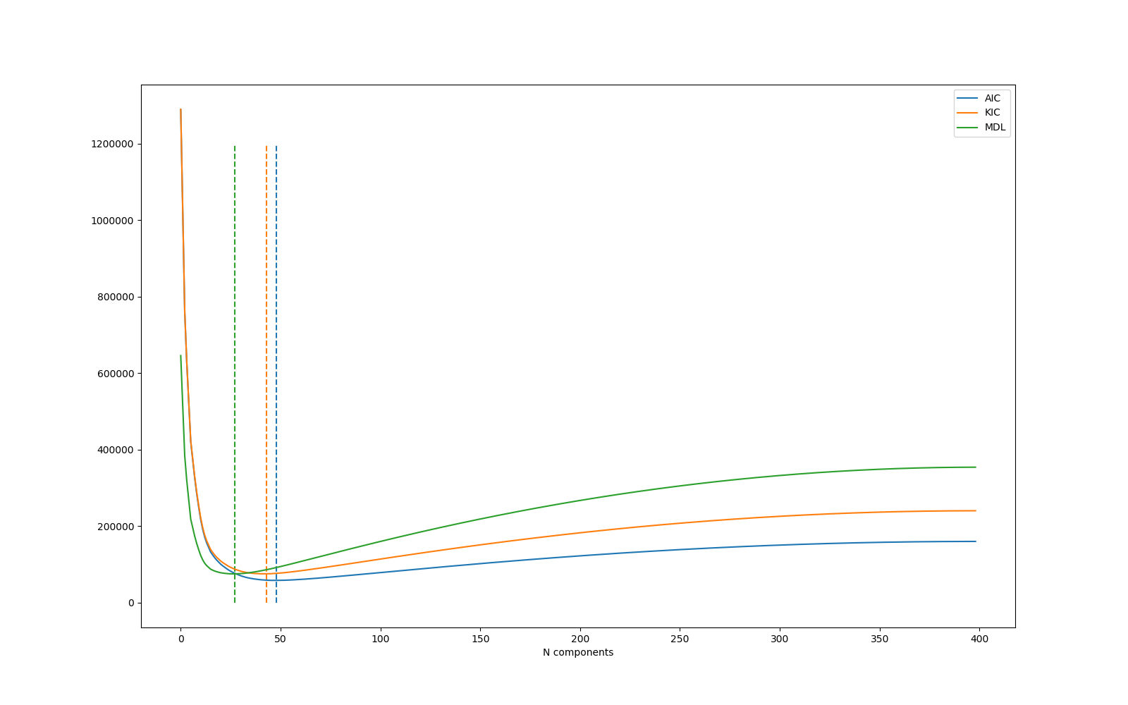
Here’s how the 3 selection criteria work on a resting-state dataset we have at BCBL.
The curves show the mdl, kic and aic values for a solution with N components (x axis). The optimal solution (vertical dashed lines) is given by the first possible solution that has a positive slope, i.e., the first possible solution with a mdl, kic or aic value higher than the previous possible solution (with one component less). The y-axis values are arbitrary.
I hope this quick iPython plot makes it easier to understand how the selection criteria work.
Edit: This is the expect behavior of maPCA. We could think of adding another 4th curve (metric) to choose an optimal solution that is more liberal. I can’t quite remember why we chose to make mdl the default option though. I guess this was the one that returned a good number of components on the data we had when we implemented this PCA method during the DC Convergence. Of course, we did not have the chance to test it on lots of data, so the more we learn about how this PCA method behaves out in the wild the better. It will allow us to tune it better for wider use.
Thanks all for explaining the pca method in more detail. I ran mdl, kic, and aic with the fmriprep explicit mask on 16 subjects (tedana_tests_txt.txt (1.4 KB) ). The average total and accepted components are mdl (32, 8), kic (48, 10.5), and aic (55, 12).
If helpful, I can send the tedana reports for each method for a low # of components subject and typical subject. To an earlier point, the adaptive mask initialized with the fmriprep bold mask does not seem overly aggressive.
Steps in progress:
I’m running meica v3.2 on a few folks now. Using afni code from a previous study in our lab for better internal comparison (although these data are from a different site, 1s vs 3s TR, etc). Will update when I have that output.
getting the matrices passed to maPCA to check mdl, kic, and aic values.
I will take a closer look at the reports to see if components are being ‘misclassified’ or differently classified for some subjects (e.g., bold-looking component in one subject is rejected in another).
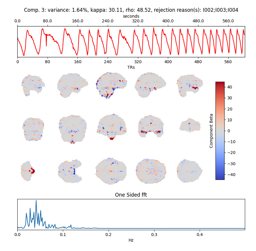
Jumping in here to draw attention to something I noticed in sub-0082 that really stood out to me - there is a strong ‘sawtooth’ pattern for the aic version, in components 2,3,8, 22, 25, 40, 51 and a similar frequency (or at least somewhat similar) oscillation in 6 and 41. This isn’t specifically tedana’s doing, but its making me wonder whats going on (and if it is contributing to your problems). Its extremely regular, and isolated to the vasculature to my eye, example:
I don’t see anything even close to this in the other dataset.
I also want to point out that the under-documented method @handwerkerd mentioned that uses a wildly different PCA selection method is still available by using ‘kundu’ as the --tedpca option (rather than mdl, aic etc). There is of course a reason it is somewhat hidden but in my hands it has had dramatic effects on the number of components - though whether that is a good thing for this data remains to be seen. It also increases the number of potential comparisons, which makes things more complicated for you.
Oh interesting, thanks for taking a look. I’m checking through the other test subjects now and will keep an eye out to see if it’s systemically related to folks with few total/accepted components. Probably worth checking the inputs too.
I saw the kundu option but I wasn’t sure at first glance how to reconcile it with the range of other options, including the meica.py scripts. Will give it another look.
@e.urunuela I added the npy files in the corresponding aic, kic, mdl directories for those two test subjects. These are older adults so they might tend to have fewer components than younger adult datasets.
@dowdlelt of my 16 test subjects I saw a few similar components in ~2 other people across mdl, kic, aic. I don’t know what to make of the potential source of the ‘sawtooth’ pattern, however. Will poke around more this week. I saw a few rejected components that could perhaps be manually classified as accepted but this was not common.
I ran meica.py v3.2 on 5 subjects (i.e., afni preproc + meica v3.2). Found comparable #s to another older adult resting-state dataset we processed this way. Average 112 total and 25 accepted, ~92% variance. afni_meica3.2_out.txt (177 Bytes)
Next, I will feed meica3.2 my fmriprep outputs just to keep the proc consistent. Then, I will run QC metrics (e.g., tSNR, FD, generate connectivity matrices) to compare meica3.2 and the tedana options. Hoping that comparison will shed light on which method works best for our data. Thanks again to all for your ongoing interest and help.
Thank you @ColleenHughes ! I’ll have a look at the curves.
For the record, yesterday we made these optimization curves more accesible in mapca with PR #43, and have started a discussion on how to make this decision more transparent in tedana itself (issue #834).
@ColleenHughes I have been looking at the code and I’m afraid I will need the mask and the 4D dimensions of your data to get the curves.
Alternatively, you could generate them yourself now that the values are accessible with mapca.aic_, mapca.kic_ and mapca.mdl_. So, you could add a breakpoint on this line in tedana and instead of running ma_pca, you can run:
Another option is that we release a new version of tedana that already saves these curves and returns the different selections as part of the PCA mixing matrix. I really don’t know how long this will take though.
Thanks for taking a look - I’m following the conversation on the github as well. I’ll try generating them myself so I know how to do it on the other test subjects.