Please discuss any issues and highlights of the tutorial content.
Best done while we are going through the notebooks the day before.
Please discuss any issues and highlights of the tutorial content.
Best done while we are going through the notebooks the day before.
Tutorial 3:
maybe it’s worth giving a reason why we resample WITH replacement. My first take is that we need i.i.d. samples, and my second take is a less appropriate example: suppose we have only two data points, then sampling without replacement will give zero confidence internal.
Tutorial 4:
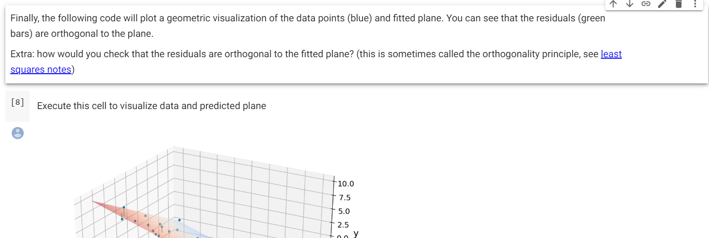
the residuals are NOT orthogonal to the plane. I know what it tries to say, but the green bars are not.
This is not really a design MATRIX. We need one row for each data instance.
Tutorial 5:
Perhaps we as TAs can show students how much the variance and bias the parameters have by plotting the learned parameters or functions.
would it be useful, as TAs, to prepare a summary of questions we think would help leading the discussion and avoiding (time-wasting) pitfalls? Would this thread be the right place to do this?
Yeah I think we can do it here, as it’s related to the content.
Okay, I’ll flag some points where I fear confusion might arise (with the caveat that I might overthinking stuff).
Tutorial 2
I think it’s mentioned in the intro video, but it’s not explicitly said here that we are trying to come up with a generative model and we assume that our data is sampled from the possible datasets that our model could generate.
If you’re still in the frame of mind where the data are given and you’re just trying to fit a line to describe it, sentences like “We want to find the parameter value 𝜃̂ that makes our data set most likely” may sound a bit weird.
Tutorial 3
As Kevin said above, why resampling with replacement?
If you want your resampled dataset to have the same size as the original, then you have to resample, but why do you want that? My guess is that if your resampled data set is smaller than the original, then the variability might be different and it will depend on the data set size, but would be good to have the correct answer confirmed.
nice one. I’m totally sunk in the Bayesian ocean…
hey @kevinwli just to check, about your remark on the residuals: the residuals are orthogonal to the regression plane, it’s just that in the plot the green lines are not orthogonal to the plane, right?
okay everyone I am confused now too  wrt tutorial 3, yeah normally you would have a finite amount of data and your resamples wouldn’t be the size of your original dataset? here’s an explanation for resampling with replacement vs without: https://stats.stackexchange.com/questions/171440/bootstrap-methodology-why-resample-with-replacement-instead-of-random-subsamp
wrt tutorial 4 the residuals will not be orthogonal unless you do PCA right? and that notebook is fitting regression? the linked notes talk about orthogonality when you do PCA. tbh I’m not really familiar with the term “Total Least Squares (Orthogonal) Regression” as it’s called in the notes (but it equivalent to PCA I believe)
Hi Carsen thanks for answering!
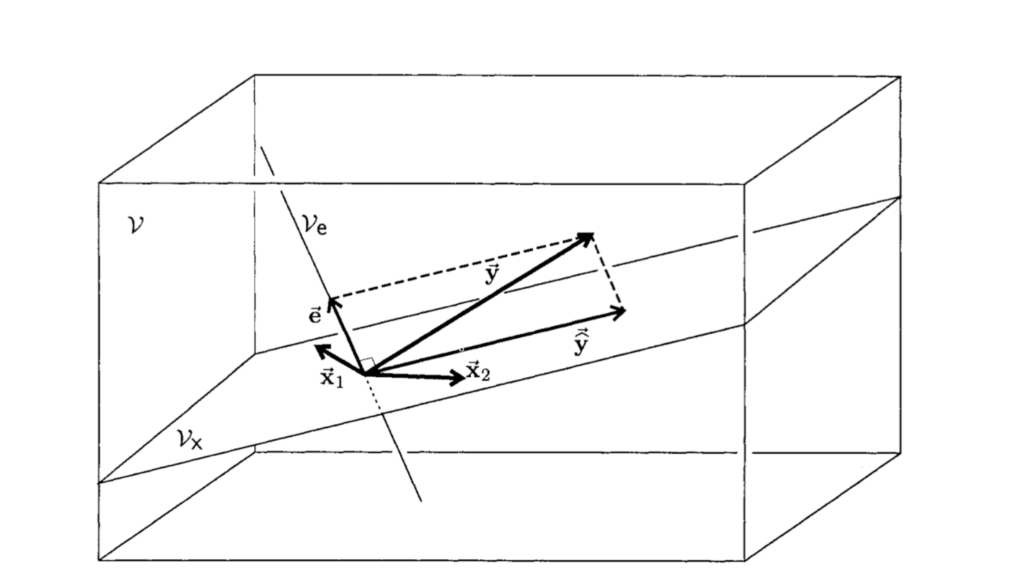
I might have got something wrong, but I think that the residuals in multivariate linear regression are orthogonal to the regression plane (at least when using standardized variables):
Here y_hat is the projection of the y onto the regression plane spanned by x1 and x2 (this follows form y_hat being a linear combination of x1 and x2).
Since the residual e is given by y-y_hat it will then by necessity be orthogonal to the plane.
This figure is from The Geometry of Multivariate Statistics which is a beautiful book on the topic, but it’s been a while since I read it so I might be wrong
Thanks for the reply.
Very briefly, the difference between each prediction y_yat and y is necessarily a vertical line, so perpendicular to the plane or the covariates/inputs (x_1, x_2). This is because the point formed by the prediction is (x_1, x_2, y_hat), and the point of the true data is (x_1, x_2, y). The plane I referred to was the one spanned by all possible (x_1, x_2, y_hat) for all possible (x_1, x_2) in R^2. And the residual is may not be perpendicular to that plane.
[In fact, the residual for each data point is simply a scalar, so doesn’t make sense to talk about orthogonality in any case… But graphically you can draw a line in that 3-D space that has a length equal to the residual]
Now, there is reason why I didn’t go into details in my last post…
The figure in your reply paints a different view of linear regression. In the figure, x_1 is a vector formed by the first dimension of all training inputs, x_2 is a vector formed by the second dimension of all training inputs, and y vector is formed by all training targets/labels.
Attempting to be artistic, I denote —x1— by the first data instance (rather than x_1 which is the first predictor in the model) as a row vector, suppose each data instance (—x1—, —x2—, etc.) has 3 dimensions, so
—x1— = [1,2,3],
—x2— = [4,5,6],
—x3— = [7,8,9],
…
—xn— = [15,16,17].`
Define the stack of the above —x--- as X, then you can then write down the residual vector for all data points as
res = (yhat - y) = (X.w - y) (1)
However, the prediction (X.w) is also the following combination:
X.w = [1,4,7...,15]^T * w_1 + [2,5,8,...,16]^T * w_2 + [3,6,9,…,17]^T * w_3` (2)
a^T indicates the transpose of a.
In this case, it is true that the residual vector yhat - y in (1) is perpendicular to the plane (assuming it exists) spanned by the two vectors in (2). In that diagram, there are two training data points, and each input has three covariates/dimensions.
The plane may not exist due to colinearity.
Yes, you can say your distribution is formed by the empirical distribution of the samples, and a sample from that empirical distribution can be obtained by sampling with replacement. You would introduce correlation without replacement. But I’m not sure if I need to get so technical to the student. @FedeClaudi’s explanation makes more sense than my second take.
yeah I think Fede’s picture explains things more clearly – linear regression is the act of projecting your data into X to get the best prediction possible, so the residuals by definition are not in the space you’re projecting into (X) and therefore the residual vector as you’ve described it Kevin is what’s orthogonal.
the vector from the plane to the data point y is not orthogonal to the plane itself and thus putting the words above that particular picture may be confusing. I’m not sure what the best way to describe this to the students is
Hi Kevin,
Thanks for posting this! It’s kind of fun to think this through carefully. Also, I could be repeating the exact same thing as you were doing here but with slightly different languages…
As @FedeClaudi metioned in his post, the least square estimation can be understooded as a linear projection because the normal equation has the exact same form as projection transformation:
![]()
However, it is important to notice here that the projection plane is defined by the column vectors of the design matrix X, rather than it’s row vectors, which represent individual data points. ![]() is defined by the coordinate of the projection in the subspace defined by column vectors of X.
is defined by the coordinate of the projection in the subspace defined by column vectors of X.
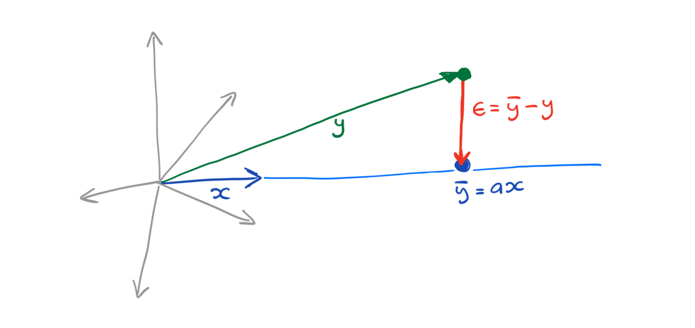
To reiterate, if we visualize the (hyper-)plane in the same space as individual data points (row vectors of X), which I believe is what this tutorial is doing here, ![]() is not the projection, and residuals are not orthogonal to the (hyper-)plane which represents the linear function.
is not the projection, and residuals are not orthogonal to the (hyper-)plane which represents the linear function.
Using one-dimensional regression as an example, the design matrix X is of size N (data point) by 1. The regression line is clearly not orthogonal to the residuals if we visualize it in the x-y coordinate system (the x-axis is defined by the rows of X, which is simply a line).
However, the column vector of X, which is an N-dimensional vector, defines the plane (line) onto which y projects. Thus, we can also solve for the slope a as the projection x.dot(y)/x.dot(x), viewing both x and y as high-dimensional vectors.
Reference: Images are stolen from this post which is a great read by itself.
Hey that’s a great reply!
That’s exactly right, and clarifies all my confusion. In the space the plots are, the residuals are not perpendicular to the regression line/plane. In the space spanned by the columns of X they are.
I doubt we will have time to go in such depth during the tutorials, but this definitively help me understand better, so thanks all of you!
Tutorial 4, video 1, around 5 min:
d should be dimensionality of y_i, not the number of input features, as it comes from assuming the noise in y Gaussian.
Moreover, for d > 1 the expression on the slide is incorrect as it should be ||y_i - X_i theta ||^2 and not (y_i - theta^T x_i)^2.
Summary of tutorial 2:
How can a function of θ “equal to” a function of y?
I would say that this is a matter of notation. Both the L() and the p() functions in this example are the same Gaussian pdf and these are 2 different notations for our Gaussian. The L() is another convention for writing a likelihood, alternative to the more traditional p().
If you think about it more algorithmically, the “input arguments” in both L() and p() are θ and x and the “function output” is y.
Haris
amazing post! and that thing they say it’s not is PCA 
it’s an application of bayes rule, see wiki section relation to bayesian inference: https://en.wikipedia.org/wiki/Maximum_likelihood_estimation
max p(theta | y, x) = max p(y | x,theta) * p(theta) / p(y)
denominator is independent of theta so =>
max p(theta | y, x) = max p(y | x,theta) * p(theta)
if we assume p(theta) is uniform then
max p(theta | y,x) = max p(y | theta, x)
(all these max’s are wrt theta)
and @NingMei to clarify your original question it’s not that they are the same but rather maximizing both of them wrt theta give the same maximal theta result
but the notebook does set them equal to each other for some reason?
Thanks!
MANAGED BY INCF