Fede, when you say we plot lambda which plot are you referring to? To me it looks like we are plotting y_t at each time point, which comes out of the Poisson pdf we are using as the likelihood, which uses lamba.
On a related note, as you write it, the correct operation is X @ theta and not X^T @ theta. In the ready code that’s fine, in the text it is written as λ = exp(X^T θ), where the dimensions do not match if X is transposed.
So I thought np.exp(X @ theta) was the definition of lambda but maybe I misunderstood something ?
I agree that Poisson comes in when computing the likelihood to fit the model, I guess I’m confused as to why np.exp(X @ theta) should be the spike count (y) instead of spike rate (lambda)? If it was a spike count, shouldn’t it be integers instead of the floats yielded by the exponential?
I think because we are using a fixed bin size, so lambda is the mean spike count of this window. `exp(X@theta)· is not the count, but the Poisson mean for unit time interval (1 bin in this case).
Not sure we need to be ‘appalled’. X^\top y is proportional to the STA, so it is pretty close to it. Given that we typically have an extra nonlinearity on top which can take care of normalisation, people (including myself) sometimes use terminology a bit more loosely. I agree with you and Anqi though we should fix it.
I agree, but in terms of teaching, we should always stick to common and more intuitive definitions. An average is better defined to be an average. And if we define them loosely we should be explicitly about it to students.
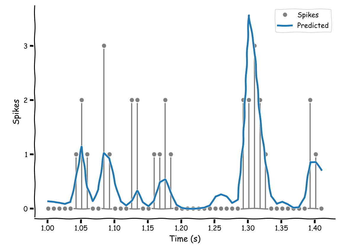
Ah yes, I see. I would say since at each time point we have an entire distribution P(y_t | x_t, θ), we chose to plot only its expected value, which in this case is λ since the distribution is Poisson. Likewise if this was a Gaussian, we would only plot its mean.
Maybe one could plot shaded areas around the blue line to represent the entire distribution (rotated vertically since y_t is on the y axis) to make a nicer but more complicated plot.
yes that’s what I was trying to get at, but I wasn’t sure if I was right.
As you say we did the same for the gaussian.
I guess we could have done a plot like for the linear regression yesterday where the entire likelihood at each time point was shown.
I have a question regarding this equation: Why is sum over lambda (as in the notebook: np.sum(lambda))
the same as the transpose of 1 (or identity matrix) ?? any clarification would be helpful. Thank you
Where we compared Non regularized weight vectors with L2 regularized ones and we changed the scale ( from -20 to 20 for Non regularized, and from -1 to 1 for L2 ) it looks like the relationship of magnitudes between each particular weight is preserved, as it has been scaled down … why is this happening?
The 1 I think represents a 1-dimensional array full of 1s and it is transposed in the equation you are referring to so it is a row array and gets multiplied by the column array that is λ. Linear algebra then says that the result should be a scalar number = 1*λ_1 + 1*λ_2 + ... 1*λ_last, which is the same as summing over all elements of λ., since each one gets multiplied by 1.
A question on “cross_val_score(model, X, y, cv=k)”. I know in the tutorials the “model” is not yet trained. But in practice can I also use a pre-trained model here?
You can pass a pre-trained model, but it will clone the estimator (dropping the weights but keeping hyperparameters) and re-train it.
What’s the answer to the bonus question in W1D4 tutorial 1. My intuition and that of the group is that we should be looking at the covariance matrix for either X or stim. Is this correct? I’m also a bit confused on why it’s the inverse of X.T @ X (inner product usually yielding a scalar) instead of X @ X.T (outer product yielding a matrix). Thoughts?
When students plotted stim @ stim.T they found that the matrix was largely the identity except that the top left was much greater. Did we make a mistake or is this to be expected?
One nice discussion question for tutorial one is why the stimuli set is a randomly flickering screen. Unlike the natural scenes retinas evolved for, this has no temporal autocorrelation. (Is that a problem? Can we safely assume that the responses to artificial stimuli are informative of natural scene responses ;))
The answer is that removing temporal autocorrelation removes collinearity in the lagged data. I’ve found it’s nice to think through this reasoning aloud with everyone.
Another thing I was told about presenting images to retinas for electrophysiological studies is that it needs moving/changing images to be able to detect the images. If you presented a perfectly stabilized image to the retina, it wouldn’t generate any response/ the image disappears.