Starting the thread here and wondering:
Why does the action play in quadratically in the cost function of T2.2?
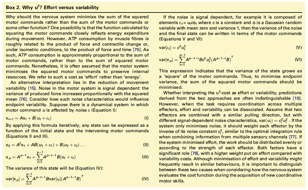
J(s,a) = sum(g- s_t)^2 + r*sum(a_t^2)
For the state it makes sense, since we want negative and positive deviations from the goal to be punished. But why not count actions in as simple discounted sum?
T1 Ex4 description of argument “belief” is wrong: the first element should be “fish on the left”, and the second element should be “fish on the right”.
But why do we want a quadratic cost function here? What is the rationale behind it?
Maybe my association is wrong, but it reminds me a lot of the regularised MSE optimisation in GLMs and I was wondering if you could also enforce sth. like sparse or smooth actions (similar to L1 and L2) or whatever one could think of as a reasonable constrain on the action space.
hmmm… my understanding is, the LSE cost function and MSE sharing the same notion; I mean, after all, both are trying to reach the min of the convex function, except that LSE for LQR is constantly updating evidence and thus taking only the sum, as for MSE is we already know all data points.
The quadratic cost function comes from the way you solve the LQR problem. When you apply LQR to a system in order to find the optimal set of actions to apply you obtain them by minimisation of the cost function. If this cost function is not quadratic (which would be the case if the actions were only summed up) you have no guarantee to find a global minimum.
To give an more intuitive explanation, let’s consider the meaning of each term of the cost function. As you said, the first one penalises deviation from the objective (both negative or positive): you want the system to be as close as possible to the objective. The second term penalises energy consumption, you don’t want to spend to much energy to reach the objective. Large positive or negative actions (in the example they are thrusts of the cat’s jetpack) will spend much energy, whichever sign is the action.
In summary, when you perform LQR (& LQG as well), you want to penalise both large errors wrt the objective & large energy consumption to reach the objective.
The control gains are computed before modelling the system; they depend only on the dynamic equations that characterize the system. They (L_t) are independent of the state which is not the case for the actions (a_t = L_t*x_t).
The high value for the control gains at the end of the movements is a consequence of the state term in the cost function and of the way the different L_t are computed (backward from the very last one to the very first one). Intuitively, this high value means that we highly want to correct any deviation observed at the end of the movement (ie. the later it happens the stronger the correction to end at the objective).
T1 Ex 3.2: The top plot shows the state, and ‘right’ is up. Bottom plot shows belief on left, and 1 is up. This is slightly confusing, and also opposite of what is shown in the next video.
In T1 exercise 4 the students are asked to complete the function policy_threshold(); what is needed is an actual if-else statement, but the commented part to modify is a single line. Given that so far the tutorials indicated if multiple lines were needed with multiple commented lines, the current form may be quite confusing for the students.
T1 Exercise 5: argument ‘measurement’ is not described in a docstring
The figures in T1 and T2 are in xkcd style, and once the students try to solve the exercises and run the cell they will lose a reference for seeing immediately if they got it or not.
Questions:
T2 Section 3 (time varying goal): I’m not sure I understand the change to the cost function. I would assume that the action cost (eg fuel expenditure) would depend solely on the final action a_t. Why should it ‘care’ about a_t_bar?
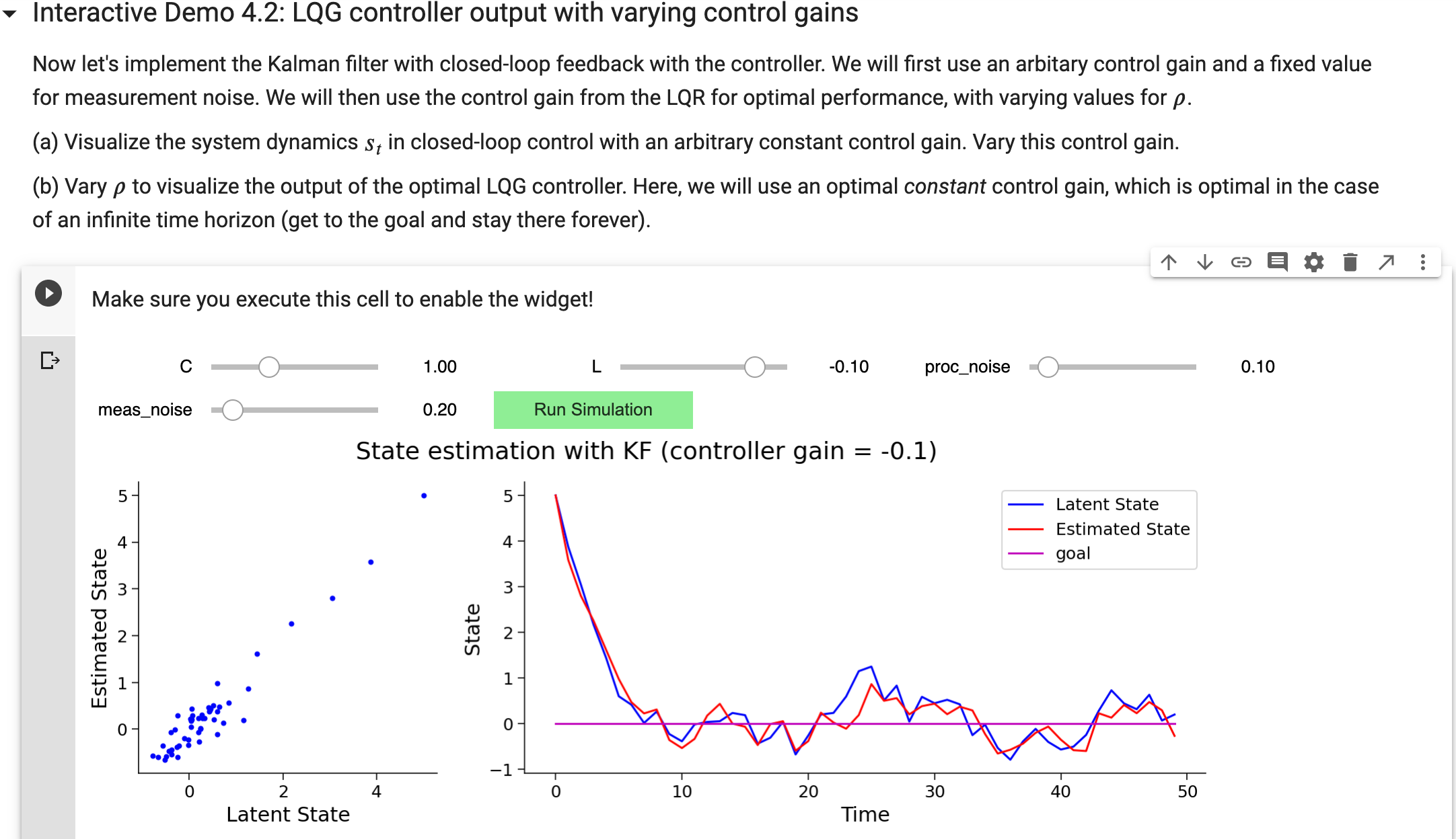
It actually seems like the effect of rho here (as seen in the interactive demo) is the opposite compared to the earlier section.
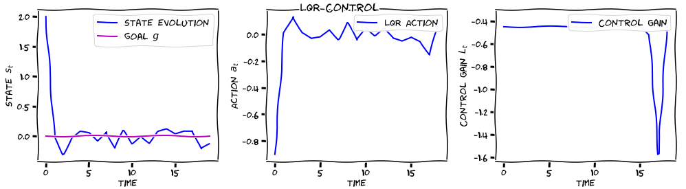
It varies strongly and sometimes even attains positive values, which try to destabilize the system… This cannot be the optimal solution! In fact, it’s not difficult to find static values of the control gain that give lower costs.
Anybody understand this? Is there a mistake in the dynamic programming solution here? Or is this behavior to be expected?
I agree with that, the part after the B (on the third line) should be the same as the line below (the control gains). I think it might explain some strange observed behaviours for the control gains (as observed by @nalewkoz below).
I think the order of tutorial 1 and tutorial 2 should be swapped in the future. Tutorial 1 (discrete state) connects better to examples in the outro and Tutorial 2 (continuous state) connects better to examples in the intro.
Sorry, the phrasing needs a little work: “We will then” was supposed to mean “in the next exercise”, where the only slider controls \rho. This one is just revisiting the Kalman filter.