AFNI 3dFWHMx output

Dear experts,

I wanted to ask a question about AFNI’s 3dFWHMx functionality.
I am using it to estimate the smoothness of my raw nifti data and I was wondering what kind of ACF model parameters as defined in AFNI (see below)

a*exp(-r*r/(2*b*b))+(1-a)*exp(-r/c) plus effective FWHM

could one expect? More specifically, I was wondering whether they should be similar to my voxel size in each direction??

Thanks a lot in advance!

Hi, @meka -

More description about the mixed ACF modeling is provided here:
FMRI Clustering in AFNI: False-Positive Rates Redux
https://www.liebertpub.com/doi/10.1089/brain.2016.0475
See Eqs. 1-3 and surrounding text for a description, and Fig 3 for a comparison with the old Gaussian modeling.

When you run 3dFWHMx, you can output a plot of the average ACF, which also shows what the older Gaussian value would be, for comparison. This is a useful way to get a sense of what the estimated “size scale” of the blur of your residuals dataset is.

The size scale of a Gaussian is typically summarized by the std dev (sigma) value, but with the mixed ACF it is much harder to do so. The mixed ACF will tend to have a weighter tail (slower decrease to zero) than the Gaussian ACF. In the above paper, it was noted that the ““Full-Width at Quarter-Maximum” (FWQM)” might be a useful way of characterizing the distance scale of the autocorrelation (because that would more appropriately reflect the tail feature than FWHM). One might look at which radius the autocorrelation is 0.5—in the AFNI Bootcamp dataset of simple task data (without REML used), that occurs about r=4.0mm for both the Gaussian and mixed ACF models (that dataset was acquired at voxel = 2.75x2.75x3.00 mm). In the Bootcamp example, the FWQM for mixed ACF was about 6.25mm (and about 5.5mm for the old/unused Gaussian approx).

I think it is hard to generalize what would be a common value mixed ACF value. It would likely depend a bit on whether you are performing REML, as well, to remove temporal autocorrelation structure. It surely also depends on acquisitions—multislice/accelerated data might have more autocorrelation structure, perhaps; field strength will matter, etc.

–pt

1 Like

Hello @ptaylor,

Apologies for my late reply- for some reason I did not get a notification of the reply!

Thanks a lot for the detailed reply, this is very helpful.
I will read your paper in detail and may possible ask a few more questions!

Thank you very much again.

Hello @ptaylor ,

Thank you very much again for the helpful reply.
I do have a few more questions and it would be great if I may have your input on them.

  1. I have highly anisotropic voxels (1 x 1 x 5 mm3), do you think this may constitute a problem for the 3dFWHMx calculations for some reason?

  2. May I ask how the radius that is used for the ACF calculations is determined? In the function help, it says: “By default, the ACF is computed out to a radius based on a multiple of the ‘classic’ FWHM estimate.” I could not understand how this value is determined, but I did notice that I cannot set a radius smaller than the radius automatically calculated by AFNI, but only higher than it. Apologies in advance if the answer is obvious and I might have missed it!

  3. In my dataset consisting of 45 participants (I have used the raw data with the detrending flag), I have compared the smoothness estimates calculated with the ACF vs the classical estimation. To my surprise, the values I obtained for the classical method were slightly and consistently higher compared to the ACF output. Interestingly, I have seen a similar pattern when I used a data set with different acquisition parameters (higher field strength, smaller voxel size). But, should this not be the other way around as the classical method underestimates the smoothness?

Thanks a lot in advance!!

Hi, @meka-

Re. Q1: Well, yes, that will probably be a somewhat odd dataset on which to do spatial calculations, such as 3dFWHMx. The spatial smoothness estimated is a function just of radius, so averaged over all angles, as it were. The strong heterogeneity of voxel dimension will create some oddities for calculations.

Re. Q2: Some gory details here. If no radius is specified by the user, then the calculation of ‘acf_rad’ is the larger of the following two quantities:
A) 2.999f * ccomb, where is geometric mean of each subvolume’s FWHM estimates; could also be the arithmetic mean of these, if the -arith opt is used.
B) 3.999f * cbrtf(dx*dy*dz), which is basically 4 times the cube root of the voxel dimensions.
… and indeed, the code is setup that one cannot choose a smaller radius than “B”, even from the command line.

Re. Q3: Well, that is interesting. I have not observed data in the wild that had that. I assume this comparison comes from the image of the red and green line (with data) being shown? Is the ACF a good fit to the data line? The “mixed ACF” model is essentially a particular generalization of a Gaussian: a weighted sum of a Gaussian and an exponential decay. I suppose it is theoretically possible to have the mixed ACF have ‘shorter tails’ than a Gaussian (or perhaps “leptokurtic” would be a more accurate term?), but I have not seen this. I suspect that the severe anisotropy might have something to do with this—but I am certainly not sure. To be sure, is this residuals that you are inputting, or some other kind of data?

–pt

1 Like

Hello @ptaylor

First of all, thank you very much for the helpful and quick replies!

Q1. I see, good to know! Actually, what we would like to do is to use this function on the same dataset (with this anisotropic resolution), before and after certain denoising steps and see how these denoising steps impact the smoothness of the data. Would this still be a valid comparison, or would you rather suggest not using this function on such data?

Q2. Thank you very much for the technical explanation!

Q3. I have observed this difference when I used the -ShowMeClassicFWHM option (please see the stdout from the function below for one participant, with the first line showing the classic/old estimation, according to the function’s help). I am interpreting these data as the classic/old estimation giving me a larger FWHM estimate – is that correct?


0.857931  0.863189   3.56048    1.38152
0.863087  0.328694   2.3981     1.0597

I used the tool both on the raw data (with the detrending option) and on data after model estimation (residuals from FSL FEAT), with very similar results. Here, I am attaching an example plot (the same subject I posted the stdout for).

I also would like to mention that, I have seen this pattern consistently across >40 subjects and also with different data-sets (e.g. 3T vs 7T data).

Thank you very much again.
Kind regards

Hi, @meka -

Q1. I would think that it would mostly make sense to calculate the smoothness of residuals, rather than the smoothness of the data itself. When we are talking about noise, that is typically what we are talking about, and that is the smoothness (i.e., spatial autocorrelation function) that is often cared about.

Q3. It is hard to judge the mixed ACF parameters without plotting them. The “show me classic” option

This might be how I would run 3dFWHMx normally—we don’t really care about the Gaussian approx anymore:

3dFWHMx                             \
    -detrend                        \
    -mask mask_epi_anat.FT+tlrc.    \
    -ACF ACF_FT errts.FT+tlrc.      \
    > acf_params_FT.txt

This would generate this text file of params: acf_params_FT.txt

# old-style FWHM parameters
 0  0  0    0
# ACF model parameters for a*exp(-r*r/(2*b*b))+(1-a)*exp(-r/c) plus effective FWHM
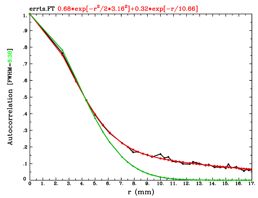
 0.676263  3.1642  10.659    8.38097

… and this figure of camparing the data points (black) with the new fit (red) and old Gaussian approx (green):


In general, the red mixed-ACF curve will better match the data points, which tend to have a heavier tail than the Gaussian can well approximate (this was a useful observation made in the Eklund et al, 2016 paper about cluster woes—AFNI implemented the mixed ACF model to be a better spatial noise fit, which seems to fit the bill).

Now, if I add the -ShowMeClassicFWHM option in order to also get the Gaussian parameters output

3dFWHMx                             \
    -detrend                        \
    -ShowMeClassicFWHM              \
    -mask mask_epi_anat.FT+tlrc.    \
    -ACF ACF_FT_W_GAUSS errts.FT+tlrc.   \
    > acf_params_FT_w_gauss.txt

… then the exact same figure gets made, and the text file acf_params_FT_w_gauss.txt would look like:

# old-style FWHM parameters
 6.13784  5.89771  5.1476     5.71173
# ACF model parameters for a*exp(-r*r/(2*b*b))+(1-a)*exp(-r/c) plus effective FWHM
 0.676265  3.16419  10.6591    8.38095

The “old-style” parameter values are not the a,b,c ones of the mixed ACF fit, and generally have very different values (they are basically the FWHM values along each axis, with the last being the “combined” or average).

So, the two sets of numbers you presented both look like “new” mixed ACF parameters, a,b,c. Here is what they look like when I plot them, calling them ‘acf1’ and ‘acf2’, respective to the order you posted them (see below for code I used):
example_mixed_acf

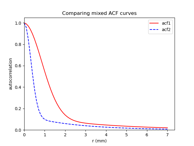
So, I am a bit confused about the two sets of parameters you are setting out—those don’t appear to me to be “classic” (=Gaussian) vs mixed-ACF values—those look much more like two sets of mixed-ACF parameters. I guess it is possible that with veeery anisotropic voxels, your “classic” parameters will be very anisotropic, as well, but I would have thought the smoothness would be larger than each voxel dimension. Your plot looks like what 3dFWHMx would give showing 1 mixed-ACF curve (red) and one Gaussian fit (green), with the data having a fatter tail than the Gaussian can manage and the ACF-fitting it well.
Therefore:
Q4. Could you please verify that the numbers you are providing are really a classic/Gaussian output and mixed-ACF fit?

–pt


Example code for plotting multiple mixed ACF profiles, plot_mixed_acf.py. Edit/add to this acf1 and acf2 variables to plot new/more curves, and execute with python plot_mixed_acf.py from a terminal, or run plot_mixed_acf.py from within IPython or Jupyter-notebook, say.

import numpy as np
import matplotlib.pyplot as plt

def make_default_r_array():

    delr = 0.1
    return np.arange(0, 7.0+delr, delr)

def mixed_acf(a=None, b=None, c=None, r=None):
    """Calculate an array for displaying the mixed autocorrelation
function (ACF) smoothness estimation parameters from AFNI's 3dFWHMx,
following the empirical relation used/described here:

    * Cox RW, Chen G, Glen DR, Reynolds RC, Taylor PA (2017). fMRI
      clustering and false-positive rates. Proc Natl Acad Sci
      USA. 114(17):E3370-E3371. doi:10.1073/pnas.1614961114
      https://pubmed.ncbi.nlm.nih.gov/28420798/

    * Cox RW, Chen G, Glen DR, Reynolds RC, Taylor PA (2017). FMRI
      Clustering in AFNI: False-Positive Rates Redux. Brain Connect
      7(3):152-171. doi: 10.1089/brain.2016.0475.
      https://pubmed.ncbi.nlm.nih.gov/28398812/

    https://afni.nimh.nih.gov/pub/dist/doc/htmldoc/programs/3dFWHMx_sphx.html#ahelp-3dfwhmx

    Parameters
    ----------
    a, b, c     : (each a float) parameter values
    r           : (array of floats) the abscissa values for plotting; default
                  is [0, 7.0] with step=0.1.

    Return
    ------
    y           : (array of float) the ordinate values, showing the 
                  mixed ACF curve; length matches that of array r.

    """

    BAD_RETURN = np.ndarray([])
    
    # check valid inputs

    if a==None or b==None or c==None:
        print("** Need to provide values of all 3 input params: a, b, c")
        return BAD_RETURN

    if hasattr(r, "__len__") :
        r = np.array(r)
    elif r == None:
        r = make_default_r_array()
    else:
        print("** Need to provide an array of values for r")
        return BAD_RETURN

    # the actual work
    y = a*np.exp(-r*r/(2*b*b))+(1-a)*np.exp(-r/c)

    return y


if __name__ == "__main__" :

    # example ACF parameter sets, output by 3dFWHMx
    acf1 = [0.857931, 0.863189, 3.56048, 1.38152]
    acf2 = [0.863087, 0.328694, 2.3981,  1.0597]

    # make array of ACF lines
    r      = make_default_r_array()
    y_acf1 = mixed_acf(a=acf1[0], b=acf1[1], c=acf1[2], r=r)
    y_acf2 = mixed_acf(a=acf2[0], b=acf2[1], c=acf2[2], r=r)

    # make plot
    
    fig1 = plt.figure( "mixed acf plot" )
    ax   = fig1.add_subplot(111)

    ax.plot(r, y_acf1, 'r-', label='acf1')
    ax.plot(r, y_acf2, 'b--', label='acf2')
    
    ax.set_xlabel("r (mm)")
    ax.set_ylabel("autocorrelation")
    ax.set_title("Comparing mixed ACF curves")

    ax.set_xlim(left=0)
    ax.set_ylim(bottom=0)

    ax.legend()
    plt.ion()
    plt.show()

1 Like

Hi @ptaylor

Thank you very very much for the helpful & detailed replies, and also for the code!

Q3 and 4.

1. I hope I did not make a mistake as I just copied the output of AFNI and did not attempt to change anything in the original function :slight_smile: . Is it possible to get two ACF profiles from 3dFWHMx function?

I would like to share the code/function call that I used, in case you would like to have a look and would be glad if you could please point out any mistake.

As I mentioned, I have seen this pattern both in the raw and denoised data (residuals after FSL FEAT) across >40 subjects, and here I am attaching the function call & results from an exemplary subject.

So this is how I call the function ( in this case, to calculate the smoothness of the residuals):

3dFWHMx -acf my_denoised_run_acf 
-out my_denoised_run_out 
my_denoised_run.nii.gz > 
my_denoised_run_STDOUT.txt

While the function is running, I see the following:


++ 3dFWHMx: AFNI version=AFNI_22.1.09 (May 10 2022) [64-bit]
++ Authored by: The Bob
e[7m*+ WARNING:e[0m   If you are performing spatial transformations on an oblique dset,
  such as my_denoised_run.nii.gz,
  or viewing/combining it with volumes of differing obliquity,
  you should consider running: 
     3dWarp -deoblique 
  on this and  other oblique datasets in the same session.
 See 3dWarp -help for details.
++ Oblique dataset: my_denoised_run.nii.gz is 2.300102 degrees from plumb.
++ removing 3 all-zero volumes from my_denoised_run.nii.gz
++ start ACF calculations out to radius = 6.84 mm
 + ACF done (0.00 CPU s thus far)
++ ACF 1D file [radius ACF mixed_model gaussian_NEWmodel] written to my_denoised_run_acf
++ 1dplot: AFNI version=AFNI_22.1.09 (May 10 2022) [64-bit]
++ Authored by: RWC et al.
pnmtopng: 43 colors found
 + and 1dplot-ed to file my_denoised_run_acf.png

And in this case, as you nicely explained, 'my_denoised_run_STDOUT.txt' looks like the following:

 0  0  0    0
 0.9169  0.607626  2.66056    1.39784

Then, I run the same function on the same dataset with
-ShowMeClassicFWHM
option with the following code:

3dFWHMx  -acf my_denoised_run_acf_classic 
-out my_denoised_run_out_classic 
-ShowMeClassicFWHM 
my_denoised_run.nii.gz > 
my_denoised_run_STDOUT_classic.txt

While the function is running, I see the following (and AFNI warns me about the ‘Classic’ model):

> ++ 3dFWHMx: AFNI version=AFNI_22.1.09 (May 10 2022) [64-bit]
> ++ Authored by: The Bob
> e[7m*+ WARNING:e[0m Using the 'Classic' Gaussian FWHM is not recommended :(
>  +  The '-acf' method gives a FWHM estimate which is more robust;
>  +  however, assuming the spatial correlation of FMRI noise has
>  +  a Gaussian shape is not a good model.
> e[7m*+ WARNING:e[0m   If you are performing spatial transformations on an oblique dset,
>   such as my_denoised_run.nii.gz,
>   or viewing/combining it with volumes of differing obliquity,
>   you should consider running: 
>      3dWarp -deoblique 
>   on this and  other oblique datasets in the same session.
>  See 3dWarp -help for details.
> ++ Oblique dataset: my_denoised_run.nii.gz is 2.300102 degrees from plumb.
> ++ removing 3 all-zero volumes from my_denoised_run.nii.gz
> ++ start Classic FWHM calculations
>  + Classic FWHM done (0.00 CPU s thus far)
> ++ start ACF calculations out to radius = 6.84 mm
>  + ACF done (0.00 CPU s thus far)
> ++ ACF 1D file [radius ACF mixed_model gaussian_NEWmodel] written to my_denoised_run_acf_classic
> ++ 1dplot: AFNI version=AFNI_22.1.09 (May 10 2022) [64-bit]
> ++ Authored by: RWC et al.
> pnmtopng: 43 colors found
>  + and 1dplot-ed to file my_denoised_run_acf_classic.png

And in this case, 'my_denoised_run_STDOUT_classic.txt' looks like the following:

 1.01437  1.09277  3.10882     1.51045
 0.916906  0.60763  2.66065    1.39784

I see the ‘old-style’ values on the upper row, but they seem similar to the lower row (at least compared to the example you kindly shared), right?

The plots automatically created by AFNI my_denoised_run_acf.png and my_denoised_run_acf_classic.png are identical. And here is my_denoised_run_acf.png attached:

2. As you pointed out, the reason for these unexpected results may be my anisotropic dateset, then? (Here, I did not attach the profiles for the values above, for the sake of brevity- please let me know if this would be helpful!)

3. And following up on the question above (and assuming that I did not make a mistake), could these results imply that I should not use this function on my dataset?

Thank you very much for your kind attention & time!
meka

Hi, @meka -

Re. Q1: I suspect it is odd coincidence that the “classic” and “mixed ACF” parameters are similar-ish. The sets of parameters represent very different things. For example, if your anisotropic voxels were anisotropic in a different viewplane, then the similarity would be broken. The first three classic parameters represent smoothness along a given axis; the first three mixed ACF parameters represent the a,b,c weights/values in the new formulation.

Re. Q2: yes, I suspect that this is another happenstance—the mixed ACF model has a notably heavier tale, and a better fit to the data.

Re. Q3: well, the dataset voxels are so anisotropic, I am not sure how good/useful an approximation “spatially average smoothness” estimates would be.

–pt

1 Like

Hello @ptaylor

Thank you very much for the replies- once again very helpful! I would like to ask my final set of questions based on your replies- I hope that is fine…

  • In this case, can I still use 3dFWHMx to compare the impact of different denoising methods on my data? In other words, I will not use the smoothness estimates for any inference but to investigate how certain denoising steps change the spatial smoothness of the data. Would this be valid?

  • If I can indeed use the 3dFWHMx function for my anisotropic dataset, would it be more reasonable to look at the classic/Gaussian estimates as I can compare the estimates for each direction (-x -y and -z) separately, instead of looking at the average smoothness estimate (which you hinted might not be ideal) or would you still go for the average smoothness computed via the mixed ACF approach?

Thanks a lot!
meka

Hi, @meka -

Re. the second point there—That thought had crossed my mind: use the directional nature of the Gaussian fits to counterbalance the anisotropy of the voxels. However, I feel like the poorer quality of fitting that gives probably defeats the point of your comparison. Having the mixed ACF is probably the better tool for comparison.

Re. the first point—I suspect that the anisotropy will “wash out” effects in the comparison, but I suppose it might be OK to do it? That is, the anisotropy will make it more difficult to see any effect in the comparison. It might still be an OK approach for doing so. (Then I wondered if using the classic parameters might “add” some extra info for the interpretation, but the unreliability of fitting the tail appropriately probably rules that out.)

Soooo, that’s a pretty waffle-y reply, I’m afraid. Booooo to the anisotropic voxels making life so complicated, but if there are large differences in the smoothness in the various processings, then you might be able to observe some. (Definitely something to note in the “limitations” portion of your study, though.)

–pt

1 Like

Hi @ptaylor ,

Thank you very much!! This was really helpful, I really appreciate it!

Yes- I have already seen a difference btw raw data vs smoothed data (the smoothness estimates were definitely higher)! But, we will definitely mention this as a limitation.

Thanks a lot again :slight_smile:
meka

Hi, @meka -

OK, cool. Maybe I would think of it this way: part of the average smoothness measure in the data will be due to autocorrelation, and part will be due to voxel inhomogeneity. It won’t be possible to partition out how much is due to each effect, but at least the inhomogeneity part shold be the same before/after or between the two different methods. So, you might still be able to observe a reduction of smoothness, likely due to processing or whatever, but you won’t really be able to quantify it in detail so easily, because of the competing effect of anisotropy—your measure would be more qualititative/approximate, I think.

-pt

1 Like

Hi @ptaylor,

I see- this is good to know!

Thank you very much!!