Yes! Nice catch. Will try to push out a patch for this shortly.
I think you are right and the ax-labels need to be swapped in the second one
Yes! If you integrate the equation, including the 1/√(2πσ²) term, from - ∞ to + ∞, it will sum to one.
However, a version that you can actually implement has two important differences from that idealized math.
- The Gaussian is only evaluated over a small part of that domain. Exercise 1 uses np.arange(-8, 9, 0.1) which is, of course, a far cry from infinity. A tiny bit of the probability mass in the tails is therefore missing.
- Even within that domain, we only evaluate it at discrete points: -8, -7.9, -7.8, … A “real” Gaussian assigns probability to all the points in between those values too.
Taking the sum fixes these problems.
1 Like
Another question - W2D1 tutorial 3 in the first exercise.
It feels like the whole tutorial is set up to deal with the gap of knowledge we have about how the brain perceives the data, but isn’t the real assumption (that we are still making) to know the distribution of the likelihood? I.e., to know how well the brain represents the data?
And doesn’t this choice eventually alter the result that we receive in the end? Because we marginalize the decisions, but these decisions change if the likelihood changes, don’t they?
Or asked differently - why do we choose sigma = 1, and what would it mean to set sigma = 2?
I think here the unknown about the brain that we are interested in is the mixing proportion of the prior, and we’re assuming we know the other parameters such as the sigmas. And in this respect indeed the goal seems to be to find the parameters which maximize the likelihood of the observed data.
This is why we need to get p(x_hat|x), which is a function of this parameter, so that we can then find the parameter value which maximizes the likelihood of the observed responses.
My current understanding is the following:
We have 3 variables of interest:
- x: the real value of the stimulus. known by experimenter, not known by subject
- x_tilde: value encoded in the subject’s brain; ‘known’ by the subject, not know by the experimenter
- x_hat: subject’s response, containing best guess about the true value of the stimulus; known to both subject and experimenter.
What happens:
-
experimenter chooses a value of x
-
subject’s perceives x_tilde
-
subject has a prior over the real values of x, p(x), and assumes a likelihood of the perception given the true value of the stimulus, p(x_tilde|x); having seen x_tilde, the subject inverts this model, computing p(x|x_tilde), the posterior belief over the true value of x
-
subject then takes the mean of this posterior belief over the value of x and gives this value as their response, x_hat
-
the experimenter assumes the subject’s prior p(x) is a mixture of known gaussians, with unknown mixing proportion, p_independent; this mixing proportion is the parameter of interest, that the experimenter wants to find;
-
the experimenter will look for the parameter p_independent that maximizes the likelihood of observing x_hat given the chosen value of the stimulus, x.
-
in order to do this, the experimenter needs to compute p(x_hat|x).
In terms of the exercises in tutorial 3 are concerned, as far as I understand they are doing the following:
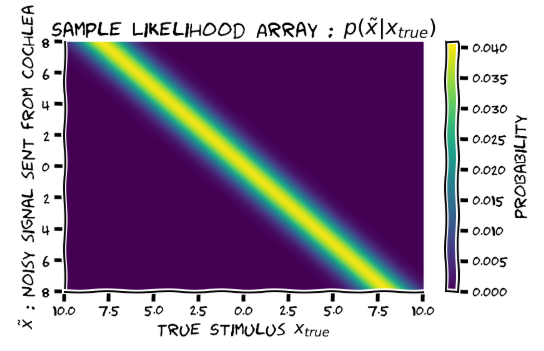
- Ex 1: getting the likelihood; the likelihood is a function of two variables, x and x_tilde; it is encoded as a 2d matrix, having dimensions #possible values of x times #possible values of x_tilde; the entry on row i column j is p(x_tilde_j| x_i)
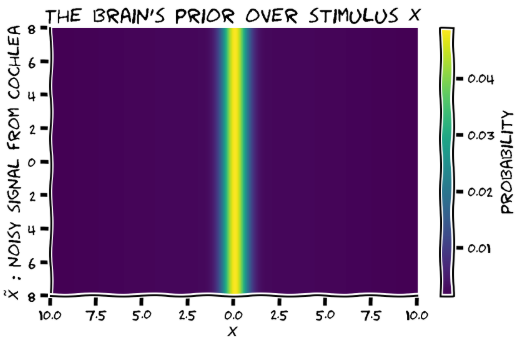
- Ex 2: getting the prior which will be combined with the likelihood in order to get the posterior over x; this has the same dimension as the likelihood matrix, but as the prior is only a function of x, it is independent of x_tilde; i think here the prior matrix should have a horizontal, not a vertical band.
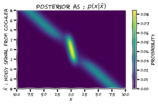
- Ex 3: getting the posterior; this has the same dimensions as the previous matrixes, and is obtained by element-wise multiplication of them; posterior[i,j] = p(x_i|x_tilde_j); my impression is that in order for the matrixes to be consistent, normalization needs to happen summing over rows, not columns;
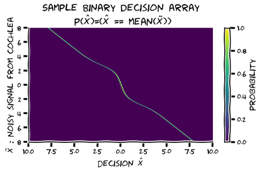
- Ex 4: computing p(x_hat|x_tilde); this will be a matrix of the same shape as above, and since x_hat is deterministic given x_tilde, it will have one 1 entry on each column, corresponding to the mean of p(x|x_tilde) for the x_tilde of that column;
- Ex 5: we are now moving on to computing p(x_hat|x), for a given fixed value of x; for this we need to integrate over the possible values of x_tilde; ex 5 aims to encode the p(x_tilde|x) that we will need for this integration;because we want the integration to be performed by again multiplying matrixes elementewise, the input array has the same shape as the binary_decision arrray, and it contains the necessary number of duplicates of a row encoding p(x_tilde| fixed x), so my impression is that it should look like a column;
- Ex6: perform marginalization over x_tilde by elemen-wise multiplication of p(x_tilde|fixed x) and p(x_hat|x_tilde); here my impression is normalization should happen summing over columns.we get a column vector encoding p(x_hat| fixed x).
I hope I haven’t mixed up rows and columns, but it’s not impossible, I’m getting quite tired 
Hope this helps, though I’m not sure what the likelihood that it does is, and how high above 0 it is
2 Likes
The prior is a function, which given a value w gives me the probability of the real stimulus being that value, without seeing any data. So as a function it is independent of the real stimulus value. But its argument is, among the variables that we have, x.
I’m afraid this sounds confusing, but can’t think of a better way to put it.
Does the subject have a prior over real stimuli, or over perceived stimuli?
I think it’s a prior over real stimuli; they have access to the perceived ones. This is what the diagram at the begining of tutorial 3 says, as far as I understand.
I think it’s a prior over real stimuli; they have access to the perceived ones. This is what the diagram at the begining of tutorial 3 says, as far as I understand.
Yes, you’re completely right. I thought that maybe the answer here was that we should think of the prior as only being defined over the variable that the subject has access to, but that’s wrong.
Still, I think the matrices are set up properly. The confusing thing is that the columns of the matrix are not always $\tilde x$: they are the variable that each distribution is defined over. So in exercise 2, look at the x axis label: it’s not $\tilde x$, it’s $p(x)$. This is saying that, for hypothetical stimulus value, the subject has the same prior, defined over the real stimulus values.
Maybe the way to put things is that the “hypothetical stimulus” axis (the rows of the matrix) is not really the same thing as $x$. You never have a distribution over hypothetical stimuli (that’s something that varies from trial to trial), but you do have a (prior) distribution of belief over $x$. This prior belief does not depend on the actual stimulus you are shown, so each row of the matrix is the same.
i think here the prior matrix should have a horizontal, not a vertical band.
As such, I don’t think this is correct.
I think that at least up to exercise 5, this is consistent. The rows are always potential locations of the actual stimulus, while the columns correspond to different things: for the likelihood they are x_tilde, for the prior they are x and for the posterior they are x|x_tilde
Yes, I agree with what you’re saying about the fact that the matrixes are set up properly if we interpret the columns differently. But then we are combining matrixes (element-wise multiplication) when their columns mean different things, and I think that they need to be consistent in order for their product to be what it is subsequently interpreted to be.
I mean, for instance, that if i want the entry i,j in the posterior matrix to be p(x_i|x_tilde_j), then this needs to be obtained as p(x_i)* p(x_tilde_j|x_i) /normalizer.
But then we are combining matrixes (element-wise multiplication) when their columns mean different things, and I think that they need to be consistent in order for their product to be what it is subsequently interpreted to be.
Both $x$ and $\tilde x$ “mean” spatial position, though. How is this different from the case where we were doing cue combination between modalities?
i’m not sure i understand what you mean, because even if x and x_tilde both refer to spatial position, they are different variables and they are not interchangeable.
but i’m getting really tired. it’s past midnight for me
if for you it’s clear what the different matrixes’ dimensions are, such that the different operations are consistent, it would be immensely helpful if you could put the info in a document and share it here. i’m sure we could all use it if you have the time to do it, that is
i’m not sure i understand what you mean, because even if x and x_tilde both refer to spatial position, they are different variables and they are not interchangeable.
I mean that $x$ = 7 and $\tilde x$ = 7 are the same point on the screen.
if for you it’s clear what the different matrixes’ dimensions are, such that the different operations are consistent, it would be immensely helpful if you could put the info in a document and share it here.
Well we’re working on pushing a last-minute fix to the tutorials that will address the typos mentioned up-thread. I think we all agree that the heatmap plots are a little confusing (I made some incorrect statements myself, reflecting my own confusion!). It’s too late to completely rework the examples, but if there are narrowly-scoped problems that can be fixed, I want to make sure that happens. I’m not sure I fully understand why you’re convinced that the prior matrix is wrong, however.
1 Like
I think a last minute fix would be very useful in this case. Please try to make the orientation of the plots identical in the videos and the code output!
I’m not convinced it’s wrong
I just can’t find a way of making it consistent with the likelihood, as it is.
As i said, if posterior[i, j] is p(x_i|x_tilde_j), then this needs to be obtained by multiplying p(x_i) and p(x_tilde_j|x_i), and it seems likelihood_array[i,j] is p(x_tilde_j|x_i). So for all j prior[i,j] should be p(x_i).
If you think there’s something wrong with this interpretations of the matrixes and point me to the correct one, then maybe that would solve the misunderstanding
My pod has students who have very little knowledge of probabilities. So here is some notes that I will use during the tutorial. I thank @elena_zamfir for very helpful discussion. Also see her post at
Disclaimer: there is quite some change to the original figures, proceed with caution.
Tutorial 1
Before going into the exercise, review the basic concepts of
- probability density/mass functions,
- joint distribution,
- conditional distribution,
- and likelihood function.
It is worth saying that we will represent a function with an array of probability mass, which can be calculated by evaluating on a grid and renormalise.Then each array will contain the probability mass at the corresponding grid (histogram if this word makes sense to students).
Section 2 after video 2
Explain the Bayes rule (probability mass version)
I would write out p(x)=N(x; m,s^2). Also, have to explain that the likelihood function is a conditional distribution with the random variable fixed, so p(sound=2|x) is the odds of observing a potentially noisy auditory stimulus of 2 given true location x.
Also worth mentioning here that if the prior is flat, then the posterior is proportional to the likelihood.
Sequential update: p(x|y=2, z=3) \propto p(x|y=2)p(z=3|x,y=2)
Introduce the idea of a visual prior
A possible story is this: let us imagine there is a flashbang going off, and we want to find its location x. Suppose that we are far away from the explosion so that we see the light first and then hear the sound.
We have no knowledge about the location before anything happened (flat prior), but the flash will update our belief about the location of the flashbang. Since the prior is flat, we have a posterior that is proportional to the likelihood of the flash, which is p(x|flahs=3) \propto p(flash=3|x)=N(flash=3|x, 1.5)
This posterior p(x|flahs=3) = N(x|flash=3, 1.5) then becomes our new prior for the subsequent sound location.
Note that, as Konrad said in a later video, the prior does not depend on any stimulus. But in this case, this prior is for the sound having seen the flash.
Exercise 2B
Explain the cue combination formula in an intuitive way (uncertainty weighted). I would skip the conjugation…
Bonus
The story before probably won’t work well for the bimodal prior, but could say now there are two simultaneous flashes, but only one of them will be followed by a bang…
Emphasise that the cause of the sudden jump is because we use an x that is most probably (MAP) to make decisions. Using the mean or median will be different.
Tutorial 2
After interactive demo 1
Rather than saying the prior switches, I would say that as the sound source moves closer to 0, the influence of the narrower Gaussian takes over and exerts a stronger pull towards the centre.
Tutorial 3
It appears that the stimulus here does not simply generate a likelihood function, but it induces noisy x_tilde drawn from a Gaussian centred at the stimulus presented. I will refer to this presented stimulus value a choice made by the experimenter, and x_tilde the noisy signal sent from the cochea to the brain. Thanks to @neurochong for pointing out.
Generative model
The tutorial draws the inference diagram for the following generative model (internal model of the world)
\tilde{x} <- x -> \hat{x} (1)
where \tilde{x} is the noisy signal sent from the cochlea to the brain, x is the true location, and \hat{x} is our motor decision. The brain has a prior p(x), and it knows the likelihood of a noisy stimulus p(\tilde{x}|x) and its decision rule \hat{x}=E[x|\tilde{x}] (\tilde{x}->\hat{x} is deterministic)
The experimenter presents a true stimulus x_true, which is never directly observed by the brain. The cochlea transmits a noisy version of x_true drawn from p(x_tilde|x=x_true), consistent with the likelihood in the brain (i.e. the brain has learnt how noisy the signal from the cochlea is, but the prior may not match the experimenter’s experimental design).
x_true ->\tilde{x} (2)
The cochlea transmits \tilde{x} according to process (2), the brain then infers the true location of the stimulus p(x|\tilde{x}), inverting the left half of the diagram in (1) above. It then uses the posterior mean to make a deterministic decision \hat{x}=E[x|\tilde{x}].
However, we do not know what the brain perceives (\tilde{x} is inaccessible), but we know it’s distribution: it is a Gaussian centred around x_true. Thus, we can marginalise out \tilde{x} to obtain the distribution of the stochastic decision p(\hat{x}|x_true).
NOTE: here the uncertainty in p(\hat{x}|x_true) is only induced by p(\tilde{x}|x=x_true)… As we will use this likelihood to fit the average behaviour of the subjects later, this is probably fine.**
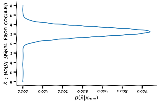
Exercise 1
The experimenter provides an x_true, this induces a noise signal \tilde{x} according to the brain’s likelihood. Note that by conditioning we are NOT conditioning the brain’s internal x, but rather the likelihood function used to generate \tilde{x} by the experimenter. The plot should then be labelled as
Exercise 2
The plot should then be labelled as
Exercise 3
Now calculate the posterior by multiplication and normalisation.
Exercise 4
Technically the action distribution should be a delta function over the decision, nonzero only at posterior mean.
Exercise 5
We now marginalise out the randomness introduced by the cochlea . The conditional distribution of p(\tilde{x}|x=x_true) should be just a marginal distribution, since x is fixed at x_true=-2.5. I’m plotting with \tilde{x} on the inverted vertical axis so that it is consistent with the previous plots.
Exercise 6
The two-d image is really the joint distribution between the cochlea signal and action, conditioned on the experimenter input x_true

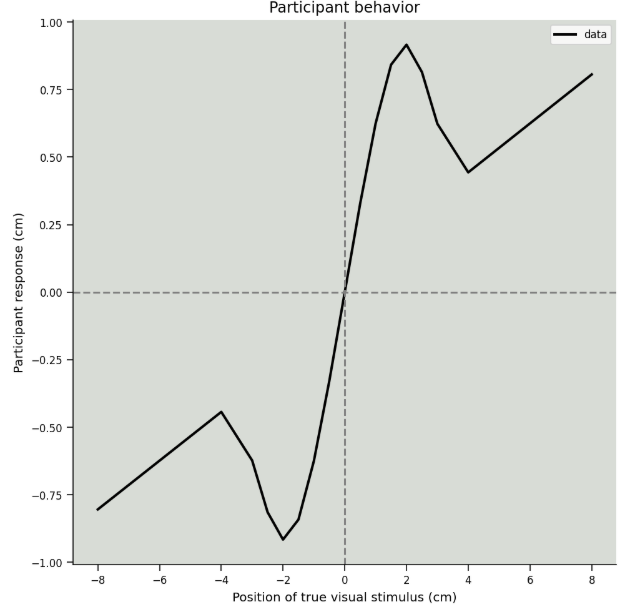
Section 7
I’m not sure why the vertical axis is labelled as a “deviation” rather than the subject response. Although this hypothetical behaviour does not make too much sense to me either way…
The notebook used to produce these figures is here.
6 Likes
I think that the main thing is to make the axis labels and figure titles more informative, eg in the prior matrix, both are stimulus location ‘x’ but one is hypothetical instantiations of it, and the other is for expressing the prior. Titles such as ‘Sample Input Matrix: $p(~x | x = -2.5)$’ (exercise 5) are very misleading. (Kevin’s post above has some great examples for fixes)
Also, I believe the axis labels are swapped in exercise 6.
As per Kevin’s post, I would change the Y axis labels of many of the heatmaps to x_tilde (‘encoded evidence’?), instead of ‘hypothetical stimulus location’, which is confusing