Different beta maps generated by nilearn and SPM

Dear Community,

I was asking myself if there would be differences between first-level results obtained by nilearn and SPM12. Therefore, I ran a very simple first-level analysis in both nilearn and SPM12. I used the same data as input for both methods, which in this case was smoothed functional MRI collected during a task in which subjects alternated between left-hand fingertapping and rest.

For the analysis, I tried to keep the same parameters in both methods, as much as possible. I used the same regressors of interest, slice time of reference, canonical HRF as provided by SPM, autoregressive model of first order, high-pass filter of 0.01 Hz. No first-level covariates were defined neither in nilearn nor SPM (to keep the computation as simple as possible).

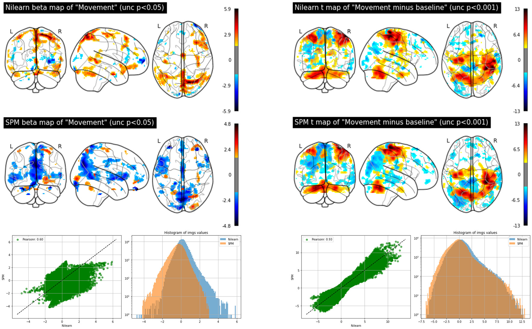
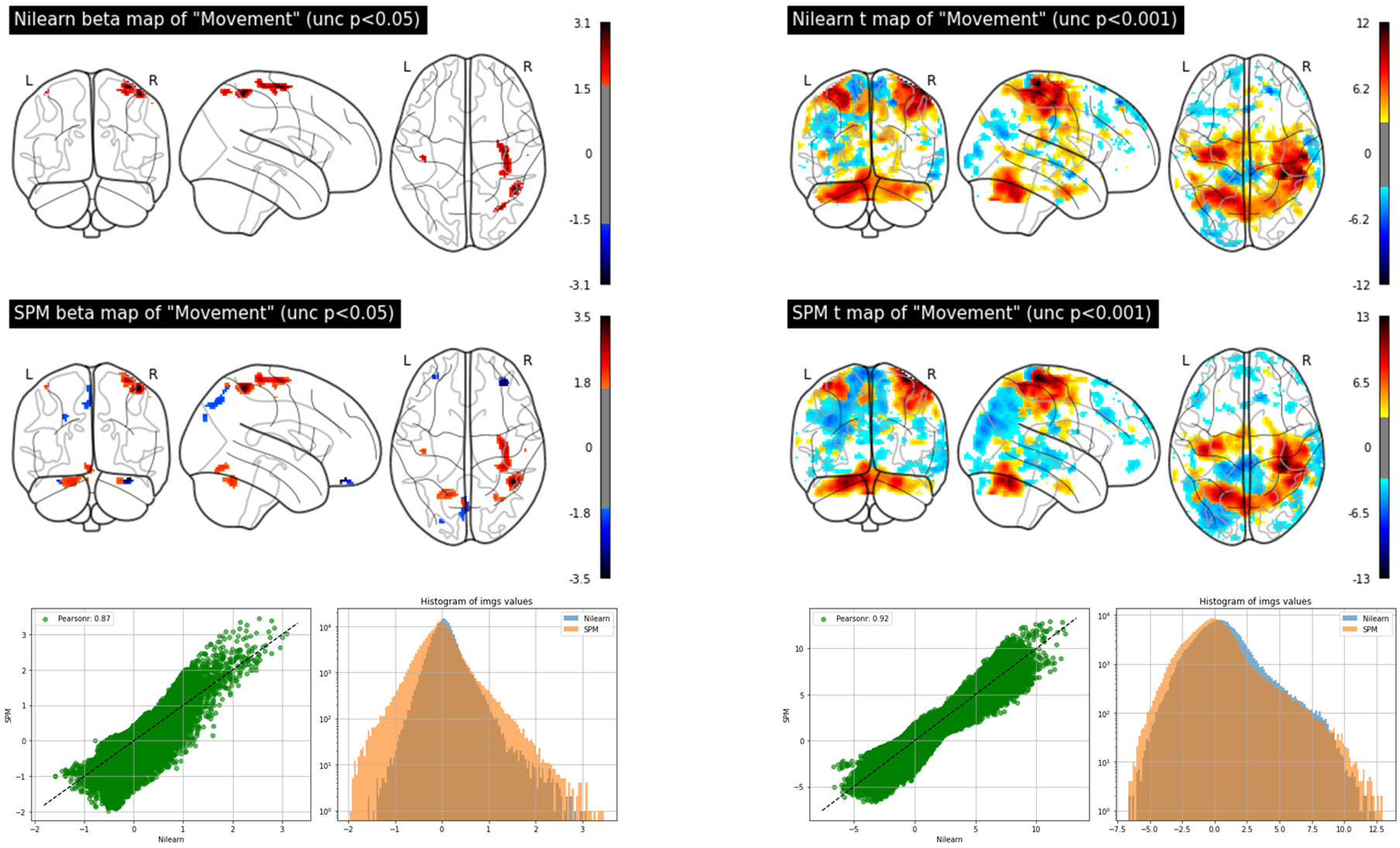
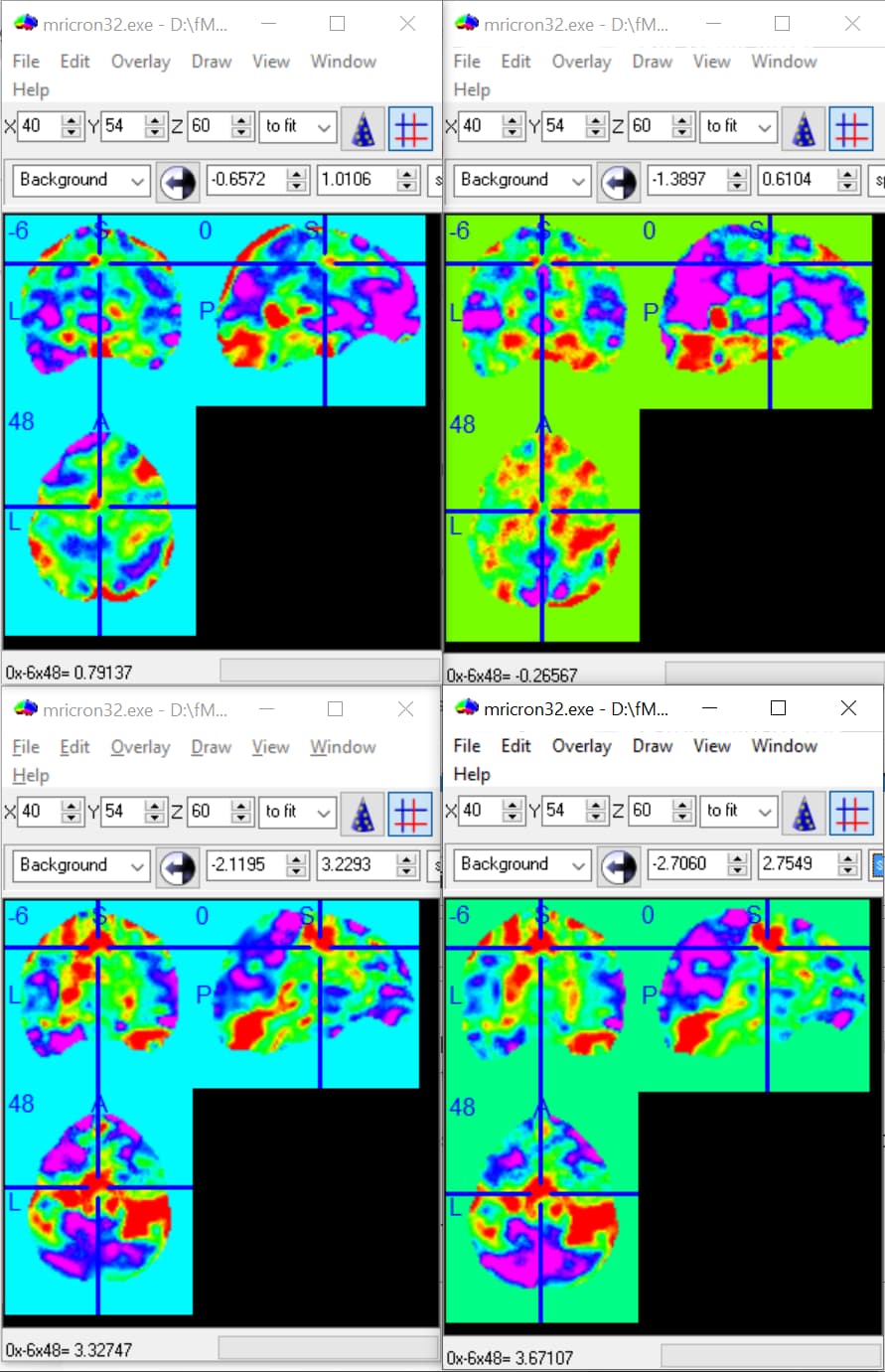
The figure below shows beta images for the regressor representing the finger tapping obtained by nilearn (top left) and SPM (top right). The figure also shows t-maps for the contrast finger-tapping minus rest obtained by nilearn (bottom left) and SPM (bottom right):

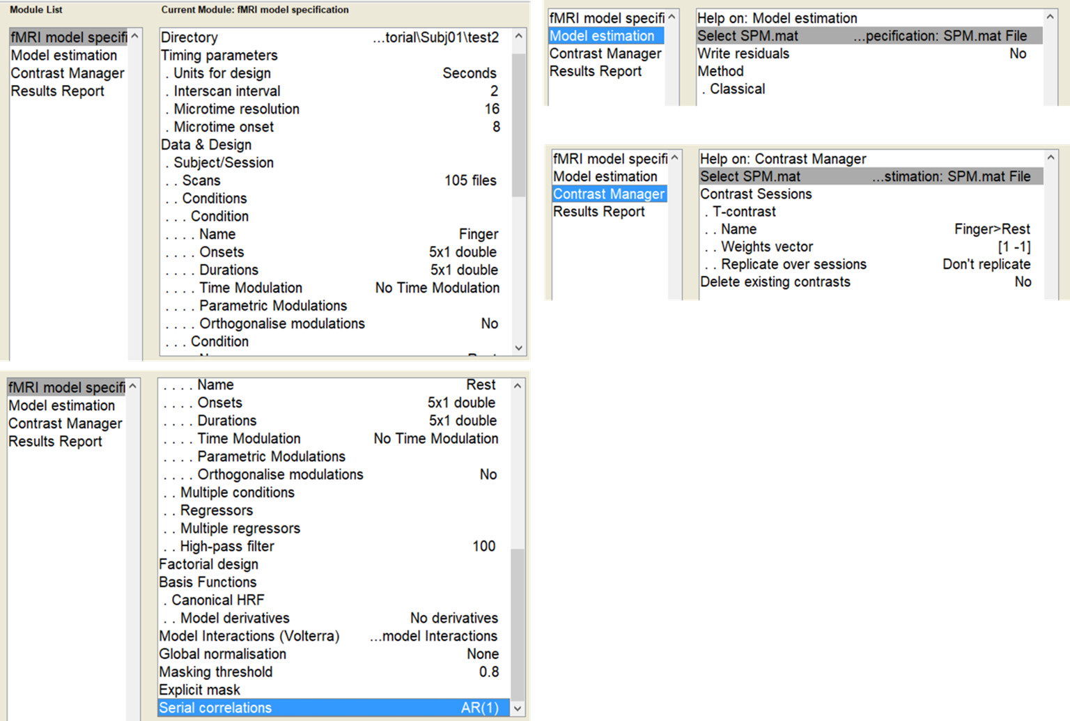
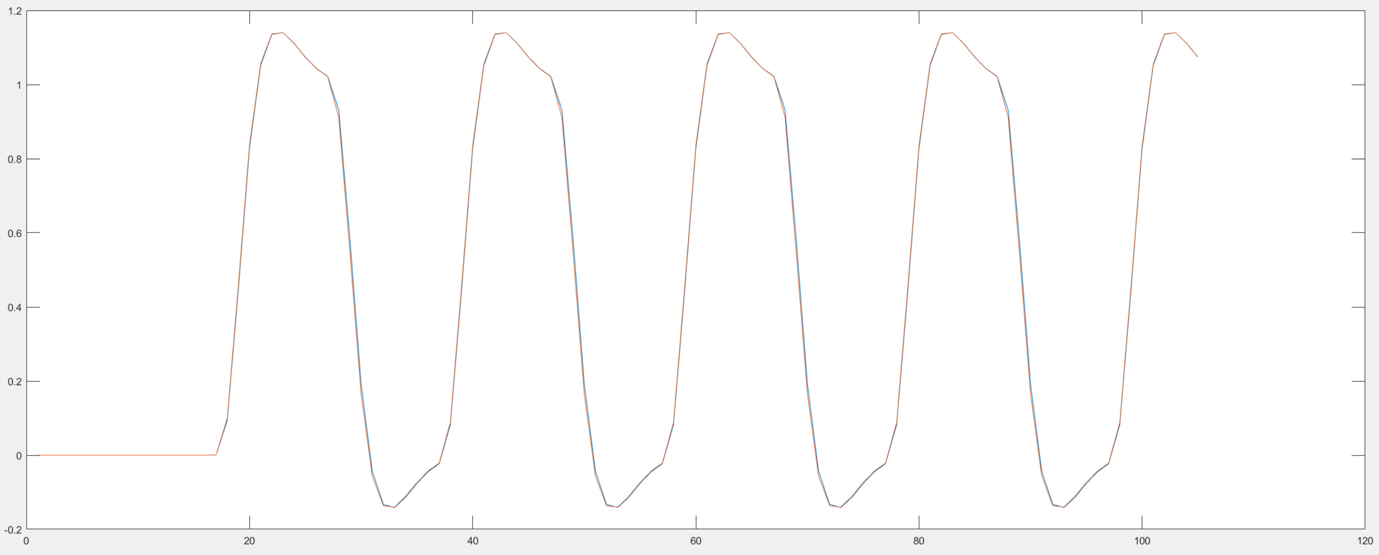
(Please find below the code I used to obtain the maps with nilearn and a screenshot of the SPM batch used)

So the conclusion is that both beta and t maps are different when obtained with nilearn or SPM and betas are more discrepant than t-maps. But one can also tell that the spatial patterns of the beta and t maps are similar by the way. First I was surprised about the results from nilearn and SPM being different, but I guess itā€™s also expected since there might be differences in the coding to compute the GLM in each method (SPM uses OLS to estimate the parameters and perhaps nilearn uses something else?)ā€¦

In any case, Iā€™m asking myself what causes these differences between methods. Or maybe itā€™s something in my code/batch that is not exactly the same in both methods? (once again, please check those below) Following up, if my codes are not equivalent, how could I write them to perform the same computation? Finally, would those differences, if they are suppose to exist, raise a concern in terms of group analysis? (for example, one takes the betas in ROI analysis and I found the beta maps somewhat different from each other).

Many thanks for any input!

Best wishes,
Gustavo

########################
Script using nilearn for first-level analysis:

from sklearn.utils import Bunch
import pandas as pd
from nilearn.glm.first_level import FirstLevelModel
import numpy as np
from os.path import join

subject_data2 = Bunch(anat = 'D:\\fMRI analysis tutorial\\Subj01\\wanat.nii', 
                 events = 'C:\\Users\\gsppa\\nilearn_data\\fMRI-motor-real-time\\sub-01\\func\\sub-01_task-motorRealTime_events.tsv', 
                 func = 'C:\\Users\\gsppa\\nilearn_data\\fMRI-motor-real-time\\derivatives\\sub-01\\func\\sub-01_task-motorRealTime_desc-preproc_bold.nii'
                 )

events2 = pd.read_table(subject_data2["events"])
events2

fmri_glm2 = FirstLevelModel(
    t_r=2,
    slice_time_ref=0.5,
    hrf_model='spm',
    drift_model=None,
    noise_model='ar1',
    standardize=False,
    high_pass=0.01,
)

fmri_glm2 = fmri_glm2.fit(subject_data2.func, events2)

conditions2 = {"movement": np.zeros(3), "rest": np.zeros(3)}
conditions2["movement"][0] = 1
conditions2["rest"][1] = 1
movement_only = conditions2["movement"]

outdir2='D:\\fMRI analysis tutorial\\Subj01\\test'
eff_map2 = fmri_glm2.compute_contrast(
    movement_only, output_type='effect_size',
)
eff_map2.to_filename(join(outdir2, "movement_only_beta.nii"))

movement_minus_rest = conditions2["movement"]-conditions2["rest"]
eff_map3 = fmri_glm2.compute_contrast(
    movement_minus_rest, stat_type='t', output_type='stat',
)
eff_map3.to_filename(join(outdir2, "movement_minus_rest_tmap.nii"))

ā€¦ and the SPM batch:

You may want to have a look at this topic: Nilearn vs. SPM very different results

Thank you, Remi-Gau. Before posting my question I had seen the topic you pointed me to. Although the OP also had different results with both nilearn and SPM, what I tried to show here was that these differences are present already in beta maps in a very simplified 1st level analysis. I tried to do as @jaetzel suggested in that post: a very simple 1st level analysis to simplify the comparison.

Also, as @bthirion suggested in that post, I took a look at the design matrices. They are almost identical for both nilearn and SPM. They have only 3 columns: movement, baseline, and constant. I show below the movement column and both lines (one for the design matrix generated by nilearn and the other by SPM) almost overlap:

Therefore, the differences in the resulting maps (see the first figure in my original post) cannot be explained by differences in the design matrix. As I posted, I tried to make additional steps of 1st level analysis as similar as possible for both methods. For example, AR(1) is specified in both methods (I actually wanted to not have this specific step for the sake of comparison, but it cannot apparently be removed from nilearnā€™s first level specification)

Therefore, I still would like to understand what leads to these different beta maps. Could it maybe be because of differences in the regression techniques used in each method?

Cheers,
Gustavo

Canā€™t you use noise_model="ols"?

Hi @tsalo,

I can, but this has to do with temporal autocorrelation in the data, not with the regression technique for the GLM. Btw, the difference still remains if I use ā€˜olsā€™ instead of ā€˜ar1ā€™

Thanks,
Gustavo

Thanks for all the extra info.

Realizing that the images you shared have slightly different scales for each software.

Maybe try the image comparison function of nilearn to get more global view of the difference.

See the section of this example that compares nilearn and FSL results:

Thanks for the suggestion, @Remi-Gau. It was indeed very useful.

So I performed a comparison between beta and t maps obtained by Nilearn and SPM. One can see it in the figure below. Beta and t maps are shown on the left and the right, respectively. Maps generated by Nilearn and SPM are shown on the top and the center, respectively. The comparison between methods is on the bottom.

One sees that indeed the t maps are more similar than the beta maps generated by each method. The comparison suggests that there might be a step in the GLM computation in nilearn that is being sort of cancelled out when the contrast is computed, but it is visible in the beta estimates for ā€œmovementā€.

Another thing is that, while in this case of SPM the average betas across voxels are slightly negative, for nilearn they are rather centered at zero. I also took a look at the beta representing baseline and I observed the same pattern. It makes me think that perhaps nilearn is also performing global signal regression in the background for the computation of betas. Or perhaps there is some sort of normalization for the beta computation in nilearn that I am not aware of (in FirstLevelModel, I set ā€œstandardizeā€ as ā€œFalseā€)? Those are just some thoughts I got by looking at the comparisonsā€¦

Checking the coding behind nilearn and SPM would be something logical to do at this point, but unfortunately I wonā€™t have the time to dive deeper nowā€¦ I would appreciate if someone could share some thoughts about how the GLM computation is conducted in both methods and how this is leading to such differences in the beta maps.

Best,
Gustavo

1 Like

The difference in betas could be due to your design - you mention Constant + Rest + Movement and if Iā€™m reading things correctly your design is nearly overparameterized. https://www.frontiersin.org/articles/10.3389/fnins.2014.00001/full see Figure 2. This can lead to unstable beta estimates, while t-stats would be less perturbed - exactly what you observer. It would likely be better to only model the Movement condition, and allow the Rest time to be captured in the automatic Constant term. Thus your contrast would be [1], as there would be no need to subtract out. The betas and t-stats would show activation relative to the implicit baseline of doing nothing

2 Likes

Thank you @dowdlelt, it was really the case that the design was overparameterized in the example I showed. Then, the methods were leading to different results in terms of beta maps because the betas were less estimable. As you pointed out, t maps were less affected. The figure below shows that, for a well parametrized design, both beta and t maps obtained by Nilearn and SPM are comparable (left: beta maps, right: t maps):

From the figure on the bottom left, I would like to follow up with another question. SPM beta map led to a larger variance of values across voxels, compared to Nilearn. Do you know why there is such a lower variance for beta maps generated by Nilearn?

Cheers,
Gustavo

I am not sure - it could be related to the high-pass filtering operations. I believe SPM uses cosines (DCT) approach - iā€™m not sure how nilearn does it, it could use polynomials, and I think there are a various approaches to apply those.

Another option is that SPM uses betas that are relative to the mean of the original signal, whereas other software (like AFNI) scales the data to have a mean 100 and constrains the HRF models to produce betas that are equivilent to percent signal change. Subtle changes in the exact data that went in, the high-pass filters, the heights of the HRF model, the level of mathematical precision, MATLAB/python differences, how AR(1) is implemented, etc could lead to greater variance but without digging deep into the code I can only speculate.

1 Like

Thank you, @dowdlelt.

It would be interesting to see a study showing the differences in the default GLM estimation settings for both methods. Also, a study showing the rate of false positives and false negatives in first level analysis for both SPM and nilearn using simulated data would be very relevant. From my example, it looks like either spm would lead to a slightly higher rate of false positives or nilearn to a slightly higher rate of false negativesā€¦ In any case, Iā€™m convinced now that both methods should lead to similar results.

Cheers

1 Like