fMRIPrep outputs very high number of aCompCors (up to 1000)

Hi fmriprep experts,

I’m using multiband acquisition, 800ms TRs, and I have several functional runs ranging from 1000-1500 TRs. For each run, I’m getting an extremely high number of aCompCors in my confounds file. I’m using ICA-AROMA as well, if that’s relevant. Is it unusual to get so many aCompCors? I am aware that there are principled ways to select how many aCompCors to include during denoising, but from reading a lot of fmriprep-related threads on neurostars, I have not seen anyone mention this many aCompCors.

Here are some examples of the output:

Thank you in advance!

Hi @ryanhucla. This won’t be the best answer as to why, but, yes, thousands per run can be expected. aCompCor is calculated by running principle component analysis on the timeseries of differently masked voxels. Principle component analysis will output as many components as there are TRs in a run (if some initial TRs are judged to be dummy scans, the exact number of components will be reduced by the number of dummy scans). However, fmriprep actually outputs 3 different sets of aCompCor components, which are based on different ways to mask which voxels are included in the analysis. You will have components that were calculated by only including CSF, white matter, or both kinds of voxels. To see which mask a particular component was calculated with, check the *desc-confounds_regressors.json file. In that json file, you’ll see a field called ‘Mask,’ which has a value of either combined, CSF, or WM. So, if there were 1000 TRs in a run, you could expect 3000 aCompCor regresssors.

That said, if you called fmriprep without adding the --return-all-components flag, then fmriprep will return fewer components. Remember, principle component analysis finds linearly uncorrelated ‘components’ that account for different partitions of variance in the data. Without that flag, fmriprep only outputs as many components as would be needed to account for 50% of the variance (shown as the blue dashed line). Without the flag, it’s hard to guess exactly how many components to expect. If the ‘up to 1000’ refers to the aCompCor components across the three masks, then this is probably about right. The number should correspond to the sum of the number of components mentioned next to the blue dashed lines in the bottom three plots you posted (92+355+378).

For picking components, the original Behzadi aCompCor implementation used the so-called ‘broken-stick’ method. As you might expect, there are many ways of picking the optimal number of components after PCA (determining how many are ‘significant’). Jackson (1993) showed broken stick way is both straightforward and works well enough. Here’s a tutorial that I found helpful while thinking about the broken stick threshold. I’m not sure how anomolous this is, but I tend to find (in a low-level visual task; 490 TRs per run) that between 0-4 components pass the broken-stick threshold (Behzadi et al. consistently found 6)

3 Likes

Hi @psadil, thank you for such a detailed reply! That makes a lot of sense, and I’ve forwarded your response to the others in my lab, as we’ve all been wondering about the details behind aCompCors in fmriprep :slightly_smiling_face:. I’m sure others that search for info about aCompCors on neurostars will find that very helpful too.

I have an interesting update – I’m using NiftiMasker to denoise my data (also detrend = True, standardize = True, low_pass = 0.08, high_pass = 0.009). I’m regressing confound regressors out of the smoothAROMAnonaggr file.

When I include the csf, white_matter, global_signal, framewise_displacement, and 6 movement parameters as confound regressors, the result looks like this:
52%20PM

When I add aCompCor50 (aCompCors that explain 50% of the variance, which, as you say, is the default output of fmriprep unless I specify the --return-all-components flag) in addition to the abovementioned confounds, the result looks like this:
49%20PM

It seems problematic to use the aCompCor50 regressors. Would I be correct in saying that this may be a case of reintroduction of noise when including aCompCors for denoising after ICA-AROMA? I’ve been reading about this potential issue in several threads on neurostars. The figures I’ve included are mean responses extracted from a region of visual cortex.

Edit: I’ve tried just adding the first 5 aCompCors. Here’s what that looks like (nearly indistinguishable from when I do not include any aCompCors):
09%20PM

And using the first 100:
02%20PM

And using the first 200:
50%20PM

Hi @ryanhucla, sorry for the slow reply. Can you clarify two points?

When you write that you “added aCompCor50” to get your second plot, do you mean that there were two separate sets of confounds that you regressed out of the data (in two steps), or did you regress out all confounds in one single step? Given that you’re talking about the reintroduction of noise, I’m assuming you did the latter (one step). That latter step would be the correct choice (unless you separately orthogonalized the regressors).

When using all aCompCor components that explain 50% of the variance, which mask were you using? (I’m not sure it matters, but if someone that knows more about AROMA chimes in the mask might be useful information)

But I agree with your inference that including the components is reintroducing noise. I’m really not familiar with AROMA; it seems like deciding which confounds to use on the smoothAROMAnonaggr data is even trickier than data which haven’t gone through non-aggressive AROMA (maybe you’ve seen them, but this thread and this one with their associated links seem particularly relevant. There may be others). ICA and PCA are closely related, in of that they’re both finding components that explain variance in the data but have different definitions of what it means for the components to be unrelated to each other. The aCompCor components are calculated prior to denoising with unaggressive AROMA, so regressing out many aCompCor components from the smoothAROMAnonaggr would reintroduce some of the variability AROMA had taken out (Lindquist et al. 2019).

To check this inference, you could make similar plots for outputs besides smoothAROMAnonaggr. E.g., I’d expect less that regressing out aCompCor50 from desc-preproc_bold wouldn’t result in such terrible voxels, while regressing out the first 5 components might have slightly more of an effect. Though, again, using the broken stick threshold I’ve often found that no aCompCor components explain significant variance, which would mean a lack of much effect from regressing out just a few components is at least somewhat likely.

When you write that you “added aCompCor50” to get your second plot, do you mean that there were two separate sets of confounds that you regressed out of the data (in two steps), or did you regress out all confounds in one single step? Given that you’re talking about the reintroduction of noise, I’m assuming you did the latter (one step). That latter step would be the correct choice (unless you separately orthogonalized the regressors).

I regressed out all confounds in one single step.

When using all aCompCor components that explain 50% of the variance, which mask were you using? (I’m not sure it matters, but if someone that knows more about AROMA chimes in the mask might be useful information)

In the figures I posted above (i.e, when I was adding 5 or 100 or 200 or all aCompCors), I was adding them in sequence (i.e., a_comp_cor_1, a_comp_cor_2, …). But it seems that if I include all aCompCors, it is using the aCompCors from the WM, CSF, and the combined mask?. Would this be redundant given that aCompCors from the combined mask contain information from both the WM and CSF masks? Perhaps this is (partially) the reason why I’m getting noise in my denoised data when using all aCompCors indiscriminately (i.e., from WM, CSF, and combined masks). However, I think another reason why I’m seeing noise is because aCompCors are derived from the unsmoothed data before it is smoothed and AROMA-corrected (as you point out in your post, and as many other posts have discussed).

The aCompCor components are calculated prior to denoising with unaggressive AROMA, so regressing out many aCompCor components from the smoothAROMAnonaggr would reintroduce some of the variability AROMA had taken out (Lindquist et al. 2019).

Yeah I’ve been reading the many threads on this potential issue. I’m aware that some tools exist to re-extract aCompCors from the unsmoothed AROMA-corrected data. But if I plan to use the smoothAROMAnonaggr output, I thnk I’d need to extract aCompCors from this file, not the unsmoothed file. Is this a correct interpretation?

To check this inference, you could make similar plots for outputs besides smoothAROMAnonaggr. E.g., I’d expect less that regressing out aCompCor50 from desc-preproc_bold wouldn’t result in such terrible voxels, while regressing out the first 5 components might have slightly more of an effect. Though, again, using the broken stick threshold I’ve often found that no aCompCor components explain significant variance, which would mean a lack of much effect from regressing out just a few components is at least somewhat likely.

That’s a good idea, I’ll try that out.

The reason why this issue I’m having is particularly strange to me is because I have used fmriprep on previous datasets and did not have issues with using the outputted aCompCors as denoising regressors (using version 1.3.2). I also had never seen so many aCompCors outputted, which is why I was asking in my initial post if that was normal. Could you elaborate on why the number of aCompCors (from either WM, CSF, or combined masks) should equal the number of TRs? I’m not sure I understand why the number of principal components should equal the number of TRs. Why would a principal component be extracted for each TR?

Thanks so much for your help, I really appreciate it as someone that does not have much experience with this. Hopefully others find this thread enlightening as well.

Paging @karofinc and @rastko here.

@ryanhucla and @psadil, could you have a look into this update to the docs (here a readable version) Karolina has been working on? Comments are welcome, and hopefully some of the questions are responded there.

If you feel like we could improve that document with your experience here, please do not hesitate to contribute.

Could you elaborate on why the number of aCompCors (from either WM, CSF, or combined masks) should equal the number of TRs?

Fair question! The answer is baked in to PCA, a widespread but also complicated concept. I think that digging in to “what is PCA” a bit would clarify some of your other questions. Unfortunately, I don’t have a good go-to link/tutorial. Maybe this one https://blog.paperspace.com/dimension-reduction-with-principal-component-analysis/? Sticking with a neuroimaging resource, maybe this video from the principles of fmri? (Anyone else reading, please chime in with your own resources).

As a brief shot at an explanation, remember that PCA (on which aCompCor is based) is defined for any matrix. One of the (many) ways to think about a matrix is as a method for storing a collection of vectors. For example, each row could represent a different dimension, and each column a different vector (whether columns are dimensions or vectors will vary). If the matrix is 2 x 10, the matrix encodes ten points in a 2-d space. Of course, the first 2-d space we imagine has axes that are oriented vertically and horizontally, which means we can imagine the matrix as showing a regular scatter plot with ten points. But axes oriented horizontally and vertically are not always the most useful or the most concise. Consider the case of all ten points falling exactly on a line with slope 1. In that case, a more useful set of axes would be one that is rotated by 45 degrees, so that what was the horizontal x-axis lines up with the line. In PCA, we call the new axes ‘principal components’ (or special vectors / eigenvectors). With this new pair of axes, the points can be completely described by where they fall on just one of the components. The component along which all the points now fall explains 100% of the variance, so might as well drop the other!

In fMRI, the dimensions are timepoints, and each vector is a voxel. It’s essentially never the case that all ‘points’ fall exactly on a line (or other high-dimensional shape). Thinking back to the scatter plot, the points might be close to a line but with some variability around that line. This means that even after you’ve found a really good way to rotate the axes, you’ll still always need at least 2 dimensions (two coordinates) to specify the position of each point. One of those dimensions might explain more of the variability in the data, but you need both to get back to the original data (to store as much information as the original matrix).

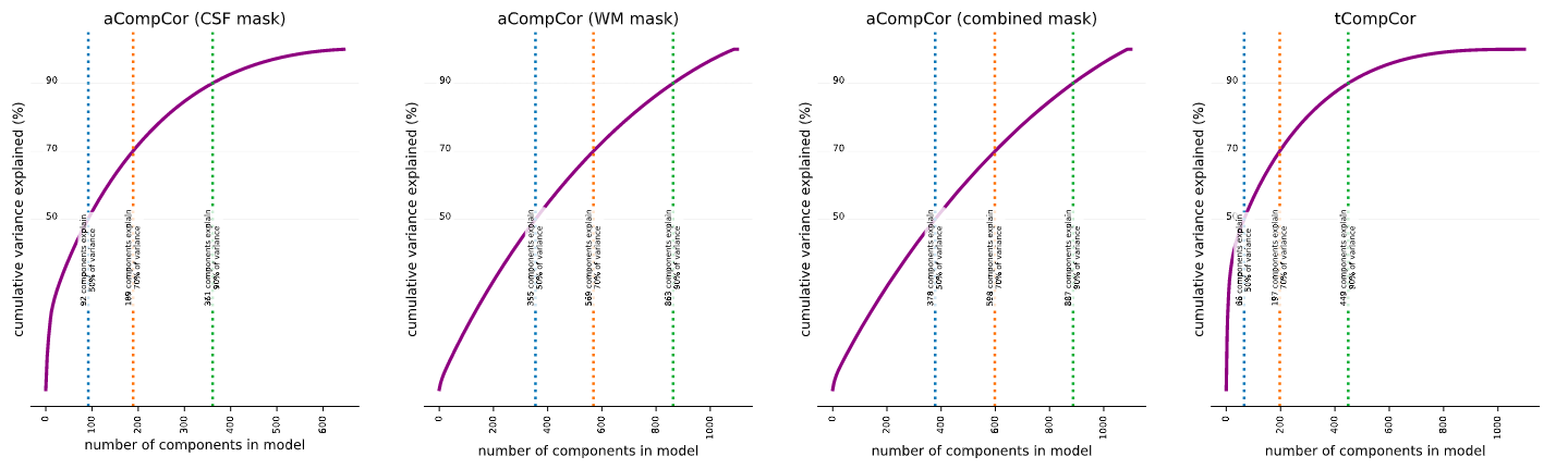
Principal component analysis may be a bit of a misnomer. The analysis stops short of decomposing the given matrix into a set of components, each of which is assigned a relative importance. It’s up to the user to make the categorical judgement of which of these components are ‘principal enough’ to include in the subsequent analyses. The thing to remember is that each TR adds a new dimension, and each voxel included in the mask is another datum in that high-dimensional space. You’d need all components if you want a complete description of the original timecourse, which is why you get 1000 components when you have 1000 TRs. But often just a few can give a pretty good description of the activity in the masked region that is systematic.

But it seems that if I include all aCompCors, it is using the aCompCors from the WM, CSF, and the combined mask?. Would this be redundant given that aCompCors from the combined mask contain information from both the WM and CSF masks?

The new docs that @oesteban linked starts to get at this. It’s not quite accurate to say that it would be redundant to include the combined mask if you’re included the WM and CSF mask, though the top components from all three likely explain similar sources of variance. The aCompCor components are calculated from each mask are calculated by running PCA with different combinations of voxels (e.g., only voxels in WM, only in CSF, or both). The best rotation that works for one set of voxels will tend not to be the same as the rotation that works for another set. e.g., imagine the scatter plot again where all ten points are on a line, but then an eleventh is way off the line. A rotation is only the ‘best’ when it enables all of the data to be concisely represented, so the best rotation will be slightly off the line with slope 1. The component that explains most of the variance will be like a regression line (still explaining a lot of the variance), with the second component still perpendicular to the first (explaining at least some of the variance). So you wouldn’t expect the top components calculated from the CSF and WM mask to necessarily match any of the top components from the combined mask (though they might be close). I’m not aware of any published, large/systematic assessment of aCompCor calculated with different masks. So if you test out different combinations, you may be in uncharted territory (which might be interesting, but likely warrants some validation).

I also had never seen so many aCompCors outputted

It’s my understanding that older versions of fmriprep only output the top 6 components (labeled 0-5), as calculated from the combined mask. I’m guessing that the reason to output only the top six was because Behzadi et al. consistently found that 6 components passed the broken stick threshold. But it seems at least plausible that the number of significant components depends on a bunch of factors (scan parameters, presence of artifacts, motion, etc), so at some point fmriprep started outputting more components calculated with different masks to give users more flexibility in subsequent analyses.

I’m aware that some tools exist to re-extract aCompCors from the unsmoothed AROMA-corrected data. But if I plan to use the smoothAROMAnonaggr output, I thnk I’d need to extract aCompCors from this file, not the unsmoothed file. Is this a correct interpretation?

I can’t comment much on the linked tools. But as a warning based on the link, the tool might not extract the principle components but instead the bold timecourses from each of these regions. If you wanted to run aCompCor, you’d then need to run your own PCA on those extracted timecourses.

hth

2 Likes

Cool! I like the added warnings. A small comment, but it looks like the a link to the ICA-AROMA paper is missing.

Thanks Patrick. That should be fixed now. I have also mentioned this thread and your detailed explanations within the CompCor warning.

If you have further comments, please do not hesitate to weigh in that pull-request conversation

@ryanhucla please check out a second round of revisions of the documentation, regarding confounds: https://10794-53175327-gh.circle-artifacts.com//0/tmp/src/fmriprep/docs/_build/html/outputs.html

I think it will be of great interest to you.

I found some missing bits of advice throughout this thread (and in our documentation):

  1. Since CompCor is run after high-pass filtering with Discrete Cosine Functions, when using a/tCompCor regressors you should also include the cosine_XX regressors in your design.
  2. Related to this, you probably should not include any of the global signals (global_signal, white_matter, csf).

Please do not hesitate to contribute to the new pull-request I’ve opened with more warnings and documentation about cosine regressors.

2 Likes