Putting mrtrix tractography into pyAFQ

Hi Everyone!

I successfully ran pyAFQ with the default tracts. However, I was unsuccessful in creating my own novel tract (the fornix) through pyAFQ. I ended up tracking the fornix in mrtrix instead. I now want to feed my fornix mrtrix tractography back into pyAFQ to get the 100 nodewise FA and MD values along the tract. I tried doing this through the “import_tract” function in the configuration file and also through API methods with no luck.

Has anyone ever been successful doing something similar to this? Is it possible for pyAFQ to re-segment a tract that I’m feeding it into 100 nodes? If so, I would love any insight or advice on how to do this.

Best,
Julia

Hi Julia,

Thanks for asking about this. I think that at the stage that you are in, you may be better off “dropping one level down”, and using the functionality for tract profile extraction that is implemented in DIPY directly, along the lines of this example: DIPY : Docs 1.7.0 - Extracting AFQ tract profiles from segmented bundles. Would that address your issue? I think that it is possible to make pyAFQ recognize your mrtrix-generated bundles as its own, but it might require some complicated definition work. So, if going directly to DIPY to get the tract profiles does the job for you, that might be a simpler route.

Hi Dr. Rokem,

Thank you so much for getting back to me! Dropping down to doing this directly through DIPY seems like it would work for what I need.

I just looked at the script, and I will try running it that way tomorrow! I just had 2 questions. Would this output a .csv file of the fa values along the tract like pyAFQ does? Secondly, would there be a way to visualize the tract in the same way as pyAFQ where I can visualize the tract and the tract profile plot on the same screen (im assuming probably not to this question but thought I’d check). If it doesnt automatically output it (specifically the .csv file) would there be a way to request that seperately?

Best,
Julia

Sorry for the slowness… Unfortunately, this will not create the CSV file for you. The DIPY version returns a numpy array that you will then need to save into a CSV file yourself. One option is to use Pandas in order to generate the structure that pyAFQ creates and then save the Pandas DataFrame object that you created into a CSV file for further analysis.

Hi Dr. Rokem,

I was able to successfully convert my .tck files to .trk and the use the DIPY script you sent to get the FA along the 100 nodes, it worked! I was also able to save it as a .csv like you mentioned.

Thank you so much for your help and for sending that DIPY resource.

I truly appreciate it so much!

1 Like

Hi again Dr. Rokem!

I wanted to follow up on this thread with a related question. I was able to use the DIPY script to successfully get the nodewise FA values and we are finding interesting results in our analysis! However, I am wondering if you know how to visualize where the nodes are starting at 0? I originally tried putting my tractography into AFQ (unsuccessfully), but I did not know if there was another way to be able to see if node 0 is starting at where the tract is seeded or ending (I’m just feeding it the tractography, not ROI’s).

For my other project where I am using pyAFQ, I checked the outputs and it looks like, for the most part, node 0 starts in the most posterior segment (but not for all), so there’s no way for us to be sure that applies here in the DIPY script.

I just wanted to check if you had any insights into how the DIPY algorithm works (like does it start in the most posterior portion or something)? Or if you have any idea how to visualize the nodes. If so I would be so grateful for any ideas you have.

Hi again Julia,

The streamlines generated by tractography algorithms don’t usually inherently have a particular direction that they are organized in. So, for example, two neighboring streamlines in a tractography may be going in opposite directions, with one that has, for example, coordinates that are more anterior followed by more posterior coordinates and the other could have coordinates that are more posterior followed by more anterior coordinates. In pyAFQ, we make sure that all the streamlines within one bundle are oriented in the same way by checking whether each streamline goes first through the first waypoint ROI in the bundle definition and flipping its coordinates if it doesn’t. So, when you observe that some bundles in pyAFQ are organized from posterior to anterior that’s because in the bundle definitions, we usually have the posterior ROI first (but you are correct that’s not always the case!). We do intend to provide a more complete description of each bundle’s orientation in the documentation, but have not done so yet.

In the DIPY example, a similar goal is achieved through this code:

qb = QuickBundles(np.inf, metric=metric)

cluster_cst_l = qb.cluster(model_cst_l)
standard_cst_l = cluster_cst_l.centroids[0]

oriented_cst_l = dts.orient_by_streamline(cst_l, standard_cst_l)

Which makes sure that all the streamlines are oriented in the same way as the centroid of the clustering procedure. However, this clustering procedure can generate a centroid that is oriented in either direction and different orientations on different runs. So, for your bundles, you’d want to figure out a way to orient your streamlines consistently across runs and across individuals. Because this depends a bit on the overall orientation of the bundle, there isn’t a catch-all solution for this, though (except to use pyAFQ whenever possible :wink:).

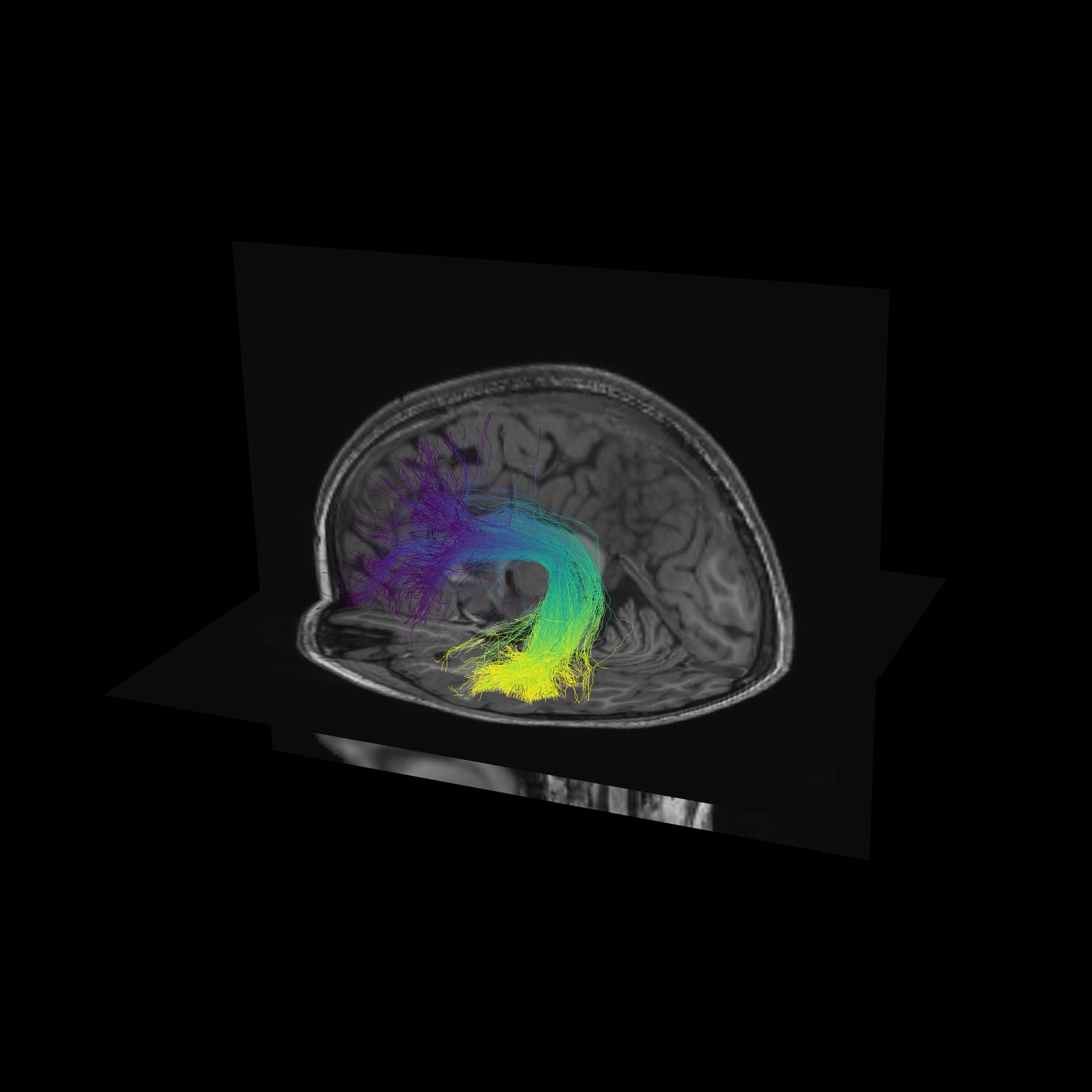
One way to verify the orientation of a particular tract profile is to visualize it. I would create a synthetic tract profile that has the numbers [0, 1, 2,...,99] in it and then plot it colorizing each of the streamlines in the bundle with these numbers. What you should see is something like this:

This was generated using the following code (which should be self-contained and downloads the data it needs):

import os.path as op
import nibabel as nib
import numpy as np

from dipy.io.streamline import load_trk
from dipy.tracking.streamline import transform_streamlines

from fury import actor, window
from fury.colormap import create_colormap

import AFQ.data.fetch as afd

afd.fetch_hbn_preproc(["NDARAA948VFH"])
study_path = afd.fetch_hbn_afq(["NDARAA948VFH"])[1]

deriv_path = op.join(
    study_path, "derivatives")

afq_path = op.join(
    deriv_path,
    'afq',
    'sub-NDARAA948VFH',
    'ses-HBNsiteRU')

bundle_path = op.join(afq_path,
                      'bundles')

fa_img = nib.load(op.join(afq_path,
                          'sub-NDARAA948VFH_ses-HBNsiteRU_acq-64dir_space-T1w_desc-preproc_dwi_model-DKI_FA.nii.gz'))
fa = fa_img.get_fdata()
sft_arc = load_trk(op.join(bundle_path,
                           'sub-NDARAA948VFH_ses-HBNsiteRU_acq-64dir_space-T1w_desc-preproc_dwi_space-RASMM_model-CSD_desc-prob-afq-ARC_L_tractography.trk'), fa_img)
sft_cst = load_trk(op.join(bundle_path,
                           'sub-NDARAA948VFH_ses-HBNsiteRU_acq-64dir_space-T1w_desc-preproc_dwi_space-RASMM_model-CSD_desc-prob-afq-CST_L_tractography.trk'), fa_img)


t1w_img = nib.load(op.join(deriv_path,
                           'qsiprep/sub-NDARAA948VFH/anat/sub-NDARAA948VFH_desc-preproc_T1w.nii.gz'))
t1w = t1w_img.get_fdata()
sft_arc.to_rasmm()
sft_cst.to_rasmm()
arc_t1w = transform_streamlines(sft_arc.streamlines,
                                np.linalg.inv(t1w_img.affine))
cst_t1w = transform_streamlines(sft_cst.streamlines,
                                np.linalg.inv(t1w_img.affine))


def lines_as_tubes(sl, line_width, **kwargs):
    line_actor = actor.line(sl, **kwargs)
    line_actor.GetProperty().SetRenderLinesAsTubes(1)
    line_actor.GetProperty().SetLineWidth(line_width)
    return line_actor


def slice_volume(data, x=None, y=None, z=None):
    slicer_actors = []
    slicer_actor_z = actor.slicer(data)
    if z is not None:
        slicer_actor_z.display_extent(
            0, data.shape[0] - 1,
            0, data.shape[1] - 1,
            z, z)
        slicer_actors.append(slicer_actor_z)
    if y is not None:
        slicer_actor_y = slicer_actor_z.copy()
        slicer_actor_y.display_extent(
            0, data.shape[0] - 1,
            y, y,
            0, data.shape[2] - 1)
        slicer_actors.append(slicer_actor_y)
    if x is not None:
        slicer_actor_x = slicer_actor_z.copy()
        slicer_actor_x.display_extent(
            x, x,
            0, data.shape[1] - 1,
            0, data.shape[2] - 1)
        slicer_actors.append(slicer_actor_x)

    return slicer_actors

slicers = slice_volume(t1w, x=t1w.shape[0] // 2, z=t1w.shape[-1] // 3)

scene = window.Scene()

scene.set_camera(position=(238.04, 174.48, 143.04),
                 focal_point=(96.32, 110.34, 84.48),
                 view_up=(-0.33, -0.12, 0.94))

sft_arc.to_vox()

scene.clear()
sl = list(arc_t1w)
for sl in arc_t1w:
    arc_actor = actor.line(
        [sl],
        colors=create_colormap(np.linspace(0, 100, len(sl)), 'viridis'))
    scene.add(arc_actor)

for slicer in slicers:
    scene.add(slicer)

window.record(scene, out_path='colored_by_direction.png', size=(2400, 2400))
2 Likes

Hi Dr. Rokem,

I cannot thank you enough for all of your insights and all of this incredibly helpful information and script!! I truly appreciate it so much. After looking closer at this script, I realized its the same as the ‘Fury’ script from the AFQ documentation which I successfully ran before (with an AFQ tract). I was nervous it wouldn’t work with my mrtrix tract but it totally did!!!

It worked so well and overlaying the ‘tube’ FA tract profile across the streamlines looks really nice as well.

Thank you so much again for responding so quickly and for all your help!

Yes! It’s the same script with the small addition of this loop:

sl = list(arc_t1w)
for sl in arc_t1w:
    arc_actor = actor.line(
        [sl],
        colors=create_colormap(np.linspace(0, 100, len(sl)), 'viridis'))
    scene.add(arc_actor)

To color the bundles from start to end. Glad to hear that it’s working well with the mrtrix bundles. If you are able, please share your image! I’d love to see what that looks like.

Hi Dr. Rokem,

Of course, absolutely! I’ll attach our images below. This mrtrix tract is going from the cerebellum to vta. We did it as is and also overlaid the FA profile ‘tube’ on top. I think they turned out really well. We truly appreciate your help so incredibly much and we love pyAFQ!


Looks beautiful! By the way, you may be interested in the new cerebellar peduncle definitions that are now part of pyAFQ based on Sivan Yossinger’s work [1,2].

[1] S. Jossinger, A. Sares, A. Zislis, D. Sury, V. Gracco, M. Ben-Shachar (2022) White matter correlates of sensorimotor synchronization in persistent developmental stuttering, Journal of Communication Disorders, 95.

[2] S. Jossinger, M. Yablonski, O. Amir, M. Ben-Shachar (2023). The contributions of the cerebellar peduncles and the frontal aslant tract in mediating speech fluency. Neurobiology of Language 2023; doi: The contributions of the cerebellar peduncles and the frontal aslant tract in mediating speech fluency | Neurobiology of Language | MIT Press

1 Like

Hi Ariel,

I remembered that I read the code you provided in this reply in DIPY examples. But I can’t find it now. Could you pls provide the link? Thanks a lot!

import os.path as op
import nibabel as nib
import numpy as np

from dipy.io.streamline import load_trk
from dipy.tracking.streamline import transform_streamlines

from fury import actor, window
from fury.colormap import create_colormap

import AFQ.data.fetch as afd

afd.fetch_hbn_preproc(["NDARAA948VFH"])
study_path = afd.fetch_hbn_afq(["NDARAA948VFH"])[1]

deriv_path = op.join(
    study_path, "derivatives")

afq_path = op.join(
    deriv_path,
    'afq',
    'sub-NDARAA948VFH',
    'ses-HBNsiteRU')

bundle_path = op.join(afq_path,
                      'bundles')

fa_img = nib.load(op.join(afq_path,
                          'sub-NDARAA948VFH_ses-HBNsiteRU_acq-64dir_space-T1w_desc-preproc_dwi_model-DKI_FA.nii.gz'))
fa = fa_img.get_fdata()
sft_arc = load_trk(op.join(bundle_path,
                           'sub-NDARAA948VFH_ses-HBNsiteRU_acq-64dir_space-T1w_desc-preproc_dwi_space-RASMM_model-CSD_desc-prob-afq-ARC_L_tractography.trk'), fa_img)
sft_cst = load_trk(op.join(bundle_path,
                           'sub-NDARAA948VFH_ses-HBNsiteRU_acq-64dir_space-T1w_desc-preproc_dwi_space-RASMM_model-CSD_desc-prob-afq-CST_L_tractography.trk'), fa_img)


t1w_img = nib.load(op.join(deriv_path,
                           'qsiprep/sub-NDARAA948VFH/anat/sub-NDARAA948VFH_desc-preproc_T1w.nii.gz'))
t1w = t1w_img.get_fdata()
sft_arc.to_rasmm()
sft_cst.to_rasmm()
arc_t1w = transform_streamlines(sft_arc.streamlines,
                                np.linalg.inv(t1w_img.affine))
cst_t1w = transform_streamlines(sft_cst.streamlines,
                                np.linalg.inv(t1w_img.affine))


def lines_as_tubes(sl, line_width, **kwargs):
    line_actor = actor.line(sl, **kwargs)
    line_actor.GetProperty().SetRenderLinesAsTubes(1)
    line_actor.GetProperty().SetLineWidth(line_width)
    return line_actor


def slice_volume(data, x=None, y=None, z=None):
    slicer_actors = []
    slicer_actor_z = actor.slicer(data)
    if z is not None:
        slicer_actor_z.display_extent(
            0, data.shape[0] - 1,
            0, data.shape[1] - 1,
            z, z)
        slicer_actors.append(slicer_actor_z)
    if y is not None:
        slicer_actor_y = slicer_actor_z.copy()
        slicer_actor_y.display_extent(
            0, data.shape[0] - 1,
            y, y,
            0, data.shape[2] - 1)
        slicer_actors.append(slicer_actor_y)
    if x is not None:
        slicer_actor_x = slicer_actor_z.copy()
        slicer_actor_x.display_extent(
            x, x,
            0, data.shape[1] - 1,
            0, data.shape[2] - 1)
        slicer_actors.append(slicer_actor_x)

    return slicer_actors

slicers = slice_volume(t1w, x=t1w.shape[0] // 2, z=t1w.shape[-1] // 3)

scene = window.Scene()

scene.set_camera(position=(238.04, 174.48, 143.04),
                 focal_point=(96.32, 110.34, 84.48),
                 view_up=(-0.33, -0.12, 0.94))

sft_arc.to_vox()

scene.clear()
sl = list(arc_t1w)
for sl in arc_t1w:
    arc_actor = actor.line(
        [sl],
        colors=create_colormap(np.linspace(0, 100, len(sl)), 'viridis'))
    scene.add(arc_actor)

for slicer in slicers:
    scene.add(slicer)

window.record(scene, out_path='colored_by_direction.png', size=(2400, 2400))

@Roger1219 : Do you mean this example?

1 Like

Thank you for your reply.
But it seems that this is not what I ever read.
I mean the code you provide in your reply to show the fiber tracts and T1 data. Is this code written by you? Or from other examples in DIPY or AFQ?

Maybe you mean this? https://github.com/yeatmanlab/pyAFQ/blob/master/examples/tutorial_examples/plot_003_viz.py

It should be easier to find this on the pyAFQ website as soon as we make a new release (which should happen before the end of the year).

1 Like

Indeed, that is exactly what I need. Thank you for your help!