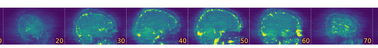
After a recent scanner issue I’ve been going back through our recent fMRI data, and I’ve noticed quite a few runs show ‘lines’ across the temporal standard deviation maps.
Hi, This could be a consequence of motion of the subject.
How are the motion traces looking for these runs where you see such a pattern?
Also parallel acceleration such as GRAPPA (that you use, if I understood correctly your post), make the acquisition more vulnerable to motion artefacts and intrinsically increase the temporal standard deviation of the fMRI runs. See this post about this effect:
How was the acquisition? slice order (interleaved or sequential)? TR (and is it a sparse sampling acquisition)? spacing between slices? Did you use Ernst angle for your flip angle?
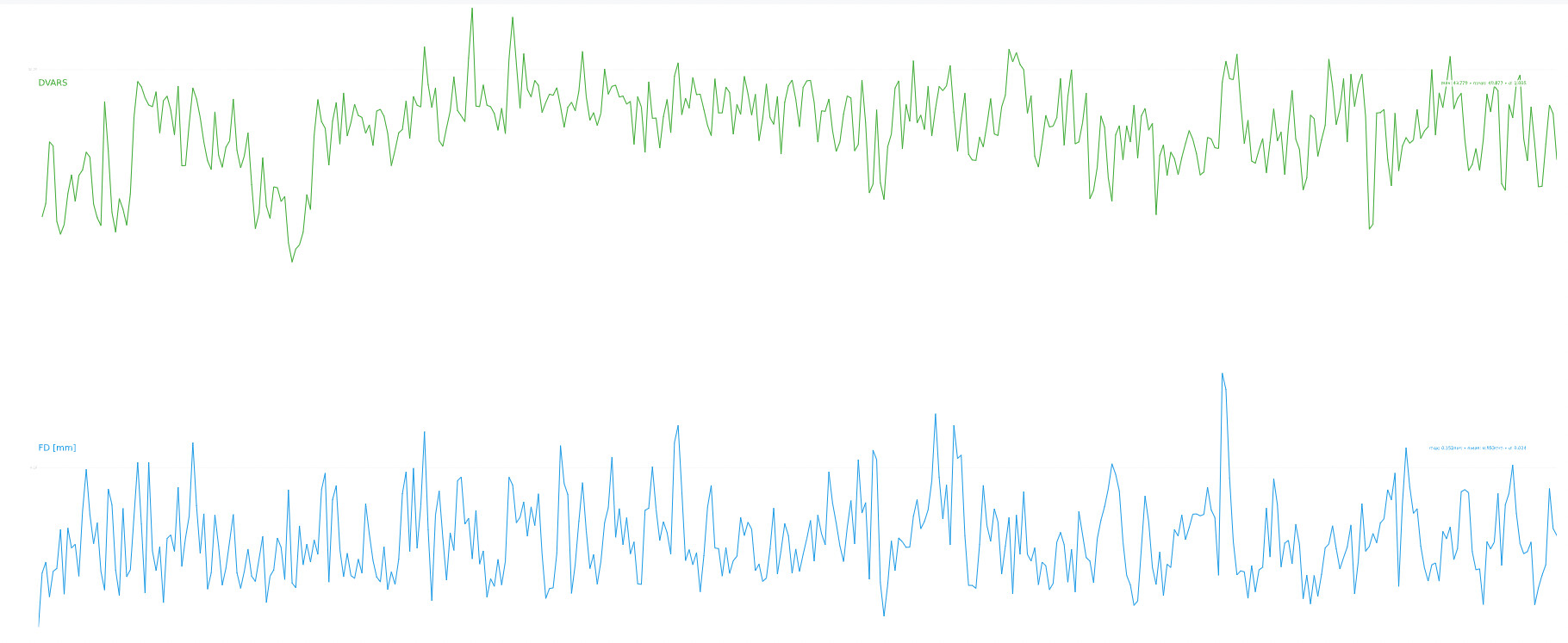
The text is very small, but mean FD is 0.05, mean DVARS is 40.876.
Slice order was interleaved. TR was 2.5s (not sure about sparse sampling). Each slice was 3mm with 0.25mm gap. We used Ernst angle to calculate flip angle.
Indeed, motion is very small. It is an interesting case.
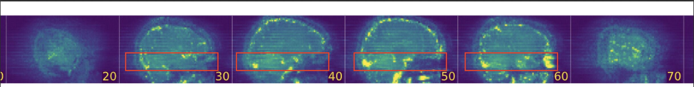
It looks like there is a band in the bottom of the brain where that effect is less visible. I have no idea why for now.
I have no definite answer, I am thinking out loud.
Did you measure this temporal standard deviation map before or after some preprocessing?
It reminds me a discussion about cross talk between slices, but that was visible in the magnitude images. Do you see this pattern in the magnitude image or in the temporal mean image?
For why I was thinking of sparse sampling fMRI, please look at the figure 2 of the following paper:
There is a long part of that paper where they investigate the origin of the slice banding pattern in the sparse sampling acquisition. I think it is worth reading that part (section 3.4), even if you are not in that case of sparse sampling acquisition. They discover an interesting interaction between the spatially non selective fat saturation pulse and the subsequently measured non-steady state water proton signal.
I don’t remember seing something similar for our acquisitions. Do you have that for all your subjects after the scanner issue?
If this is now systematic and you have the possibility to try to do some tests at the scanner, you could try:
to reproduce the same thing on a phantom
change the acquisition order to ‘descending’ or ‘ascending’ for another run.
remove the fat sat and see the impact of the banding
I would encourage you also to look at the unprocessed data as a movie along different view (in fsleyes for instance) and check if you detect something.
Thanks for these suggestions, they are very helpful!
The scanner issue we had was that the Z gradient rectifier broke last week. But this scan (and some others) were taken a year before so I’m not convinced that this issue is related to that. I’ve not yet got data after the scanner was repaired, so I will check that as soon as I can.
This temporal standard deviation map was calculated before any preprocessing was applied. I’ve checked the temporal mean image and there are no similar artifacts there. Also the raw data on movie mode shows nothing obvious. The other strange thing is it is not present for all participants, or even all runs for the same participant.
I’ve checked and this was a continuous acquisition, but it does look similar to the artifacts in that paper so I wonder whether there are similarities regarding the fat saturation pulse. I guess it’s somewhat reassuring that statistically there was little difference between the scans with slice banding and without.
Thank you for the testing suggestions! I will also see if I can try the sequence on a different scanner and see if we get the same artifact.
Thank you for your feedback. It is definitely an interesting artefact. Since you are using a continuous acquisition, I think you are not in a similar case as in the paper described above, where the artefact was related to non-steady state magnetization.
Speaking about artefacts visible in the temporal standard deviation map only, this artefact hunt reminds me about another chase, well described in this other great blog: MVPA Meanderings: Holy crescents, Batman!. It is not the same pattern, but it is also something visible only in the temporal standard deviation map.
Regarding the motion pattern for those subjects where you see this artefact, it may be interesting to look at the absolute motion curves that give sometimes more information than the FD curve.
Have you tried to looks at the ICA components that can be produced by MRIQC? (--ica option)
Perhaps you can more insights on this particular pattern looking at those components?
Temporal standard deviation maps shouldn’t have such prominent stripes. That they show up as flat in the raw (not-preprocessed) images certainly suggests that they are related to the acquisition, and look rather too prominent to ignore. If they’re clearest in the runs with the least movement, I’d suspect that they might actually be present in all cases, but be “blurred” by movement and preprocessing and so less easy to spot in higher-motion runs. If you look at axial slices do you see brighter and darker slices in single frames (meaning moving up and down in a single image)? Or perhaps flashing if you look at a single slice when viewing the run as a movie?
You might get a quick diagnosis from an MR physicist on twitter ; this seems like the sort of thing that someone would recognize at a glance.
I checked some data gathered from another scanner and the banding is not present there using similar acquisition parameters. Also, since the scanner has been repaired the banding has gone.
Our local physics team thinks maybe the banding was due to a problem with the Z gradient leading to inconsistent slice selection.
I can see brighter and darker slices in single axial frames. Would this be consistent with inconsistent slice selection?
Thank you for this interesting feedback and thank you Jo for bringing your thoughts!
What you report Nathan makes total sense. For axial slices the Z gradient is used for the slice selection, so it is safe to think that a defect on the Z gradient may have produced this kind of temporal instabilities, visible on the temporal deviation maps. This effect must have been producing variable cross-talk between slices (partial saturation of spins from one slice because already excited from a previous slice that was not appropriately prescribed) explaining also the brighter and darker slices in single axial frames.
Good catch and hopefully now you are out of problem after the repair of the Z-gradient.
Thank you again for sharing, this may be useful at some point to somebody else encountering a similar issue!
Glad to hear that the scanner is fixed, though that doesn’t help with your already-collected data. Do you think the affected data will be usable? It seems like it could be, but you’ll have to do quite a bit of checking.
 ; this seems like the sort of thing that someone would recognize at a glance.