We found it gave unreliable results; ie run it twice on same data and get quite different results. we switched to fsl-fix and found that it does a very good job, provided you have 20 or so subjects and a bunch of time spare to establish a training set for your protocol!
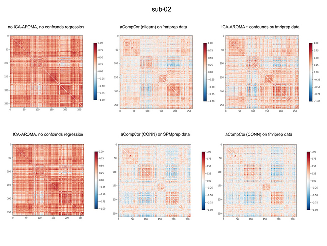
Few months ago we did some simple comparisons of individual correlation matrices calculated on data obtained from fmriprep and SPM, and denoised in CONN toolbox and nilearn using confounds from fmriprep’s .tsv table. First, we noticed that correlation matrices from not denoised data (*_preproc.nii.gz) and output from ICA-AROMA (non-aggressive) were not very different in most cases. Second, when applying denoising (WM and CSF) on output from ICA-AROMA, histogram of correlation values was still little left skewed. For aCompCor we also included as confounds WM/CSF and 6 motion parameters. See example result attached. If I only find some more time, I will summarize this findings better.
I visually inspected output from fmriprep and ICA-AROMA results look fine.
We run fmriprep on data obtained on GE scanner, no multiband.
Thank you very much for sharing your results, @karofinc . Did you happen to correlate functional connectivity with an estimate of subject motion in the scanner (e.g., mean Framewise Displacement)?
We didn’t, but I will do this together with summary of our findings. I should have it within two weeks. Thanks!
This reminds me of a problem we have been working; see:
Later preprocessing steps can reintroduce previously removed artifacts if one isn’t careful. For example, temporal filtering after motion regression, can reintroduce the motion into the data. The amount depends on the interaction between the two filtering operations, not on the complexity of the motion regression. This could perhaps explain your findings.
Interesting observation @Alex_Fornito . I’m suspecting it will have to do with instability of the ICA decompositions. Are you limiting the dimensionality at all? We found it beneficial to limit the number of components to 100-150 for high volume multi-band data.
This was some time ago, so can’t remember off the top of my head. I don’t think we explicitly limited the #dimensions.
These might be helpful:
Figures 4-6 from https://www.sciencedirect.com/science/article/pii/S1053811917302288?via%3Dihub#ab0010
Figure 6 from https://academic.oup.com/cercor/article/27/9/4492/3056417#113569675
It really seems that the optimal preprocessing strategy may be dependent on the question that is being asked. When looking at individual or group differences it looks like using more motion parameters and scrubbing, or using ICA-AROMA (with our without GSR) may be reasonable bets. If anyone had other resources suggesting optimal preprocessing streams I would be all ears, particularly ones that synced nicely with fmriprep.
Thank you all for the feedback.
Thanks @mtnhuck , I modeled my preprocessing pipelines largely after the Ciric et al. (2017) paper, from what I understand, the approach I have taken differs very little from that of Ciric and colleagues. Yet, my results differ substantially. I am in the process of testing different software (i.e., FSL’s fsl_regfilt instead of AFNI’s 3dTproject for the regression) and will report back as soon as I have results.
Very interesting paper @fMRIstats , I will have to give a more detailed read to more deeply appreciate. Currently, I am using AFNI’s 3dTproject which I believe conducts a regression of nuisance variables (e.g., motion parameters), spikes (i.e., single TRs), and trends (0th, 1st, 2nd order) in one model. However, after extracting mean time-series for ROIs, I apply a temporal filter (butterworth, highpass = .009 Hz, lowpass = .080 Hz) in Matlab before computing temporal correlations. Does this seem to be problematic given your experience? In reading the abstract, it appears as though it might…
With regards to ICA approaches, ICA-AROMA does not seem to handle the “zebra-patterned multiband motion artifact” (e.g., see Figure 8 in Griffanti et al., 2017; https://www.sciencedirect.com/science/article/pii/S1053811916307583 ) that I see in some cases. I wonder if in your experience @Alex_Fornito , ICA-FIX can handle this in the classifier if given appropriate training data? Thanks for the suggestion @mmennes , I used the default component dimensionality selected in fmriprep, which may be a source of issue, but at a glance, for my data (TR = 1.5s, length = 400), the number of ICA components is seldom more than 150. Do you think this is too large of dimensionality? Is there a suggested way to check?
Thanks again all.
Scott
@burwell, my understanding is that if you use 3dTproject with the -passband flag specifying your bandpass range, it should simultaneously perform temporal filtering and nuisance regression, as recommended in paper by @fMRIstats. You do not need to do temporal filtering afterwards if you use that flag.
its been a while, but in our experience it does pretty well.
This is an interesting thread and I’m curious to hear what may explain the anomalous results…
I just wanted to mention that the use of 3dTproject will probably yield rather different results than fsl_regfilt given the ‘non-aggressive’ approach that the latter typically adopts. It’s also worth noting that ICA-AROMA has been vetted primarily using the non-aggressive method.
Briefly, the main difference is whether voxelwise BOLD data are regressed on noise components alone (this is what you’re doing with 3dTproject, I believe) versus regressed on all timecourses from the ICA decomposition (the non-aggressive fsl_regfilt approach). In the fsl_regfilt case, the partial regression coefficients reflect the association of a noise component with the data in the presence of both noise and ‘good’ components. The signal to be removed is computed by multiplying the partial coefficients for the noise components by the timecourses for those components, summing the results, then subtracting this from the BOLD timecourse.
Here’s a small R function that does the same thing as fsl_regfilt. y is a voxel timecourse, X is the time x components matrix from (melodic) ICA, and ivs is a vector of numeric positions in X containing flagged noise components.
partialLm <- function(y, X, ivs=NULL) {
  require(speedglm)
  #slower, but clearer to the math folks
  #bvals <- solve(t(X) %*% X) %*% t(X) %*% y
  #pred <- X[,ivs] %*% bvals[ivs]
  m <- speedlm.fit(y=y, X=X, intercept=FALSE)
  pred <- X[,ivs] %*% coef(m)[ivs]
  return(as.vector(y - pred))
}
This is a strong contrast to the 3dTproject approach where the association between noise and non-noise signal sources is not considered, which could lead to removal of potentially useful BOLD variation.
Hope this helps clarify at least one part of this anomaly.
Very nice explanation of what is going on. This approach divides the variance shared between noise and signal into the the noise and signal coefficients. In other words some, but not all and not none of the noise/signal shared variance will be removed from the data. How do you think this approach would compare to orthogonalizing the noise components against signal components prior to regression (in other words making sure none of the noise/signal shared variance is removed from the data)?
Thank you again @fMRIstats for sharing your insightful paper. I have re-run a couple versions of my pipeline to test the effects of sequential (regression of 6 motion parameters, followed by high-pass filter) versus simultaneous (regression of 6 motion parameters and stop-band regressors) de-noising procedures.
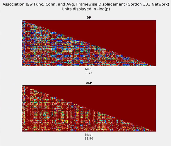
Sequential motion regression–> temporal high-pass .009 Hz:
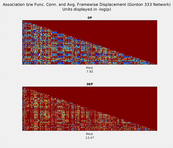
Simultaneous motion+stopband (.009 Hz) regression:
As evidenced by the plots, regardless of the sequential vs. simultaneous method taken, the association (-log[p]) between Functional Connectivity strength and Frame-wise Displacement is greater when the 6 motion regressors are included (labeled “06P”) versus when they are not (“0P”). I do not point this out to disagree with the arguments made in your paper, but rather I don’t think this to be the bases for the anomalous findings in my data.
I wonder if spatial smoothing (and/or ROI time-series extraction, another form of spatial smoothing) following motion/stop-band regression might introduce noise? E.g., although the time-series of one voxel might be orthogonal to motion parameters, might averaging it with its neighbor reintroduce some association with motion? Is the “best bet” to smooth before motion regression? Or rather to conduct the motion regression on the extracted ROI time-series? I am working on a way to test my speculations, but if anyone has any insight into this question, it would be greatly appreciated!
Just a side note: you can limit the number of ICA components in fMRIPrep using --aroma-melodic-dimensionality 150
Interesting! Thanks for checking. I’ll have to think more about this…
Thank you @Michael_Hallquist for the detailed explanation on the non-aggressive (vs. aggressive) regression filtering processes conducted in AROMA. True, the 3dTproject program does not take into account the “signal” components in the regression model and only regresses out “noise” components.
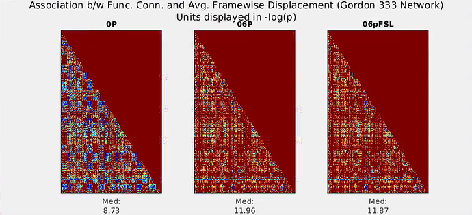
Nonetheless, @jforawe’s above point (posted on 2018-08-30) about functional connectivity from the “06P” model (6 motion parameters as “noise”) having greater association with mean Framewise Displacement than the “base” model (i.e., first 5 volumes removed; 0th, 1st, and 2nd order detrend, filter) is the most puzzling. So, part of my confusion is due to issues independent of AROMA. IF the voxel-wise BOLD time-series are indeed made orthogonal to the 6 motion time-series, wouldn’t one expect functional connectivity (inter-voxel correlation) to have a reduced association with Frame-wise displacement (a linear combination of the 6 motion parameters)? (Note: I’m not directing this question at you specifically, just reiterating the confusing aspect  ). I found a related 3dTproject discussion on the AFNI discussion boards from fall 2016, but I’m not sure it’s the same issue I’m seeing. I also re-ran a highly similar preprocessing pipeline, where detrending was done (AFNI’s 3ddetrend), followed by regression of 6 motion parameters using FSL’s fsl_regfilt, followed by smoothing (AFNI’s Merge), and get basically the same result.
- 0P, no regression conducted, “base” model
- 06P, regression in AFNI
- 06pFSL, regression in FSL
As I posted earlier today, I wonder if part of the issue stems from the fact that, at least with the “6P” data, spatial smoothing (and ROI time-series extraction) occurs after the noise-regression (I’m not sure when its done in the AROMA sequence), and I am curious if spatial smoothing among voxels might reintroduce some of the motion associations? I have no evidence of this now, but hope to in time.
Did you ever figure out what was going on here? I have not run into this issue in my own analyses.
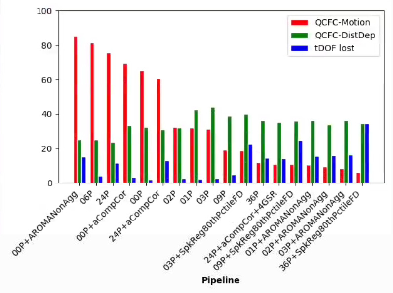
At the moment, I have not found clarity as to what is going on. After several denoising approaches (re-computing the non-aggressive AROMA output, voxel- vs. ROI-wise denoising), I still observe patterns similar to my original post. For the below-explained models, the associations between quality control functional connectivity (QCFC, temporal correlations among Gordon’s 333 ROIs) and motion (mean Framewise Displacement) are worst (largest) for the simple ICA-AROMA model, 6 motion parameter model, etc. Even more peculiar, the association between QCFC and motion for these models is greater than the “00P” model, where only highpass filter cosines and non-steady state outliers were regressed. (I’m developing Python scripts at https://github.com/sjburwell/fmriprep_denoising , if anyone is interested in testing on their own data.)
The below denoising pipeline models regress out the following:
00P: highpass filter cosine functions, non-steady state outlier TR
01P: 00P+global signal
02P: 00P+white matter, csf
03P: 01P+02P
06P: 00P+motion parameters
09P: 03P+06P
24P: 06P+1st difference and quadratic expansion of the parameters
36P: 09P+1st difference and quadratic expansion of the parameters
03+, 09+, 36+SpkReg80thPctileFD: these models, plus spike regression of high motion TRs
00P+, 24P+aCompCor: inclusion of the aCompCor columns
00P+, 01P+, 02P+, 03P+AROMANonAgg: non-aggressive AROMA filtering, done using fsl_regfilt; for 01, 02, and 03 models, global signal, white matter, and csf were estimated after the initial AROMA filtering.
In the above, the red bars pertain to the percentage of edges in the 333 node network significantly related to motion (p < .001), the green bars pertain to the absolute-valued distance-dependence of the functional connectivity (x100, to keep on the same scale as the other bars), and blue bars pertain to the percentage of temporal degrees of freedom lost.
In general, my results are consistent with papers by Ciric et al., (2017) and Parkes et al., (2018), but they do not report 00P models, so I cannot say whether that aspect is consistent or not.
When you do the FD - network edge regressions, is this an across-subjects regression?
What do you think you would see if you instead measured FD-ROI regression coefficients within subject time-series as in ROI ~ 1 + FD
I usually find these to be substantially reduced after aCompCor and motion parameters.
