Unusual High Functional Connectivity Values for Multi-echo fMRI Data

[AJavan]

Dear all,

I have processed multi-echo resting-state fMRI images (three echoes per scan) using fMRIPrep (V.24.1.0) on singularity. To remove dummy volumes and perform further denoising, I applied the following steps on fmriprep outputs:
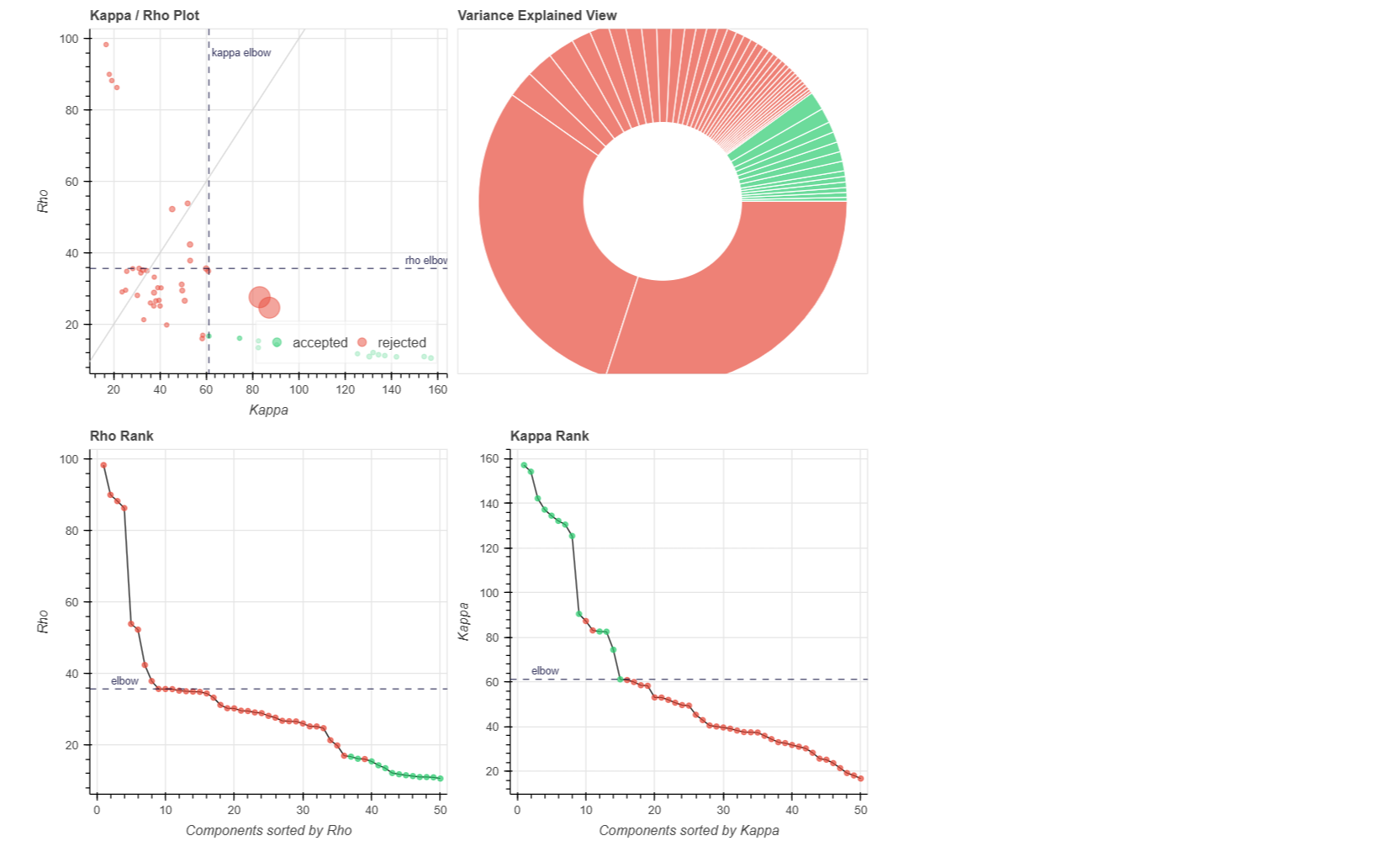
(1) removed the dummy volumes from the echo-wise files, (2) ran tedana (V 24.0.2) on those trimmed files, (3) removed the dummy volumes from the MNI-space optimally combined file from fMRIPrep, and (4) used tedana ICA components to denoise the trimmed MNI-space file as discussed and suggested on a (former topic on Neurostarts). I took the non-aggressive approach with no confounds (just the rejected components) to apply denoising on the data using Nilearn. After denoising, I extracted the timeseries from the Schaefer 7-200 parcellation and computed the corresponding functional connectivity matrices. However, the resulting connectivity matrices exhibit unusually high values, which seem unexpected to me. I’d appreciate any insights on whether such high connectivity values are typical given this type of sequence and denoising approach. If they are expected, are they considered acceptable? If not, what strategies could be used to address this issue?

Attached below are the codes used for these steps, including the application of Tedana on fMRIPrep outputs to obtain the main mixing matrices necessary for further image denoising:
tedana_wave2.txt (3.7 KB)
Code for applying tedana denoising using nilearn:
denoise_nonaggr_MTL0002.txt (2.8 KB)
Code to extract connectivity matrices from the Schaefer parcellations:
connectivity_schaefer200_wave2_MTL0002_FU84.txt (2.1 KB)

Here is the connectivity matrix csv file:
connectivity_nonaggr_schaefer200_MTL0002_FU84.txt (978.4 KB)
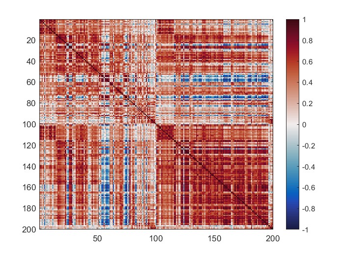
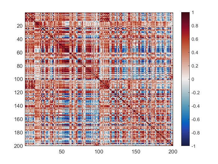
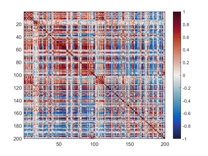
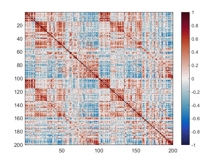
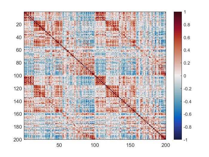
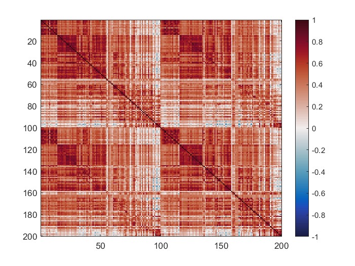
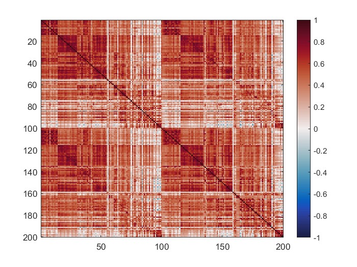
The mean connectivity value of the whole matrix is 0.42, and here is the plotted functional connectivity matrix.
The following image is the plotted connectivity matrix in matlab.

Many thanks in advance,
Ali

[handwerkerd]

Hi Ali,

tedana should remove noise, but there’s no expectation that it will remove all noise sources. There’s a good chance it won’t remove artifacts with BOLD weighting. For example, if your volunteer was breathing slowly and deeply or doing spontaneous breath holds, that could create a global artifact that’s BOLD weighted.

It’s unclear if this is an issue with a subset of runs or with your entire dataset. If it’s a subset of runs, I recommend looking at the *_tedana_report.html file. A guide on how to interpret it is here: Outputs of tedana — tedana 24.0.2 documentation Given you’re showing a large global artifact, I’d expect at least one relatively high variance component that was accepted, but where the time series and/or component map looks like an artifact. If this is happening in just a couple of runs, you can use ica_reclassify to fix these problems. (Ideally make a protocol for looking at the reports and consistent rules for when to change classifications).

If this is happening on many runs, you look at the reports, and see consistent characteristics of bad components that were accepted, it might be possible to tweak the accept/reject decision tree to address this issue. (It could also be a sign of an underlying data problem)

Hope this helps

Dan

[AJavan]

Hi Dan,

Many thanks for your

@handwerkerd

It’s unclear if this is an issue with a subset of runs or with your entire dataset.

Yes, this pattern of high connectivity values were prominent across several randomly selecetd runs connectivity matrices.

@handwerkerd

Given you’re showing a large global artifact, I’d expect at least one relatively high variance component that was accepted, but where the time series and/or component map looks like an artifact.

Looking at the reports of those individuals, apparently no high varaiance accepted component existed with a similar profile of an artifact. Please find a copy of the Kappa/rho and the explained variance figure below for your reference and to ensure my interpretation. Also, I have not noticed this scenario in other visualized reports either, so I would say there is not a misjudgement on component classifications that could doubt the decision tree selection.

@handwerkerd

if your volunteer was breathing slowly and deeply or doing spontaneous breath holds, that could create a global artifact that’s BOLD weighted.

I am also attaching below, the fMRIPrep report figure on the FD and DVARS plot for this check:

Would you think that integrating the noissance regressors (motion, WM, and CSF) with perhaps the Demo external regressors single model decision tree could be beneficial in this regard? And if so, since the decision tree have not yet been validated, is there any special checks to ensure its performance on our data? Additionally, how different would it be to use a decision tree that takes into account the regressors with using the default decision tree and including those regressors along with the rejected components as confounds when applying the ica denosing from the already estimated tedana components?

Thank you so much for your time and guidance,
Ali

[handwerkerd]

Looking at your report, one thing I notice is that 80-85% of your explained variance is rejected. This isn’t implausible, but it’s on the higher end of plausible. Compare this to some of your other runs. Perhaps this run is just particularly noisy and that makes it harder to isolate relevant signal?

Looking at your fMRIPrep report, I do see systematic DVARS fluctuations (maybe at breathing rate?) and some spikes that appear in the carpet plot, so there clearly is global noise.

In the scatter plot, I see a bunch of green dots with rho values about the rho threshold and kappa values below the kappa threshold (dashed lines). Those are the ones that are most likely to be incorrectly accepted & can merit further inspection. If you run tedana with --tree minimal most or all of those will be rejected. It might be worth trying that and comparing results.

The external regressors functionality works, but the benefits of the included decision tree have not been systematically evaluated yet. I very much welcome people testing it out. The underlying logic is to reject components that significantly correlate with external regressors and the external regressors also model at least 50% of the variance of the component’s time series. I consider this a reasonable hypothesis for a useful rejection criterion, but it really needs testing for a range of regressors & data sets.

That said, if you give tedana external regressors as input, you can apply classification tags to components even if you don’t change their classifications. That means, you’d be able to inspect the components in the report and the hover text will show which ones significantly correlate with motion, respiration, CSF, etc.

Also, several groups have been evaluating external regressors, they’ll be giving a brief presentation at a multi-echo fMRI zoom meeting on Friday, March 14, 2025. More info here: https://groups.google.com/g/tedana-newsletter/c/gmkvjP1MIyU

Dan

[AJavan]

Hi Dan,

Thank you for your comments, I have tested the suggested potential contributing factors and here are the details:

@handwerkerd

Compare this to some of your other runs

I checked the reports of several runs and participants, similar pattern of the low explained variance by BOLD components was prominent to the similar extend across all.

@handwerkerd

If you run tedana with --tree minimal most or all of those will be rejected. It might be worth trying that and comparing results.

As you expected, using --tree minimal, removed all the suspecious components and the rejected/accepeted components’ rho/kappa values lied within the expected ranges with regards to the rho/kappa thresholds. You may find tedana’s report attached below, and the code here:
tedana_wave2_tree_minimal.txt (3.6 KB)

Further, I denosied the trimmed (dummy removed) MNI-space optimally combined image from fMRIPrep, using “denoising with component” of tedana (applying the mixing matrix obtained from tedana to the image)
denoise_nonaggr_MTL0002_NoConfounds.txt (3.1 KB)
The recomputed the connectivity matrix from this step can be found below:

@handwerkerd

The external regressors functionality works,

Further, I included confounds when denoising with components. denoise_nonaggr_MTL0002_confounds.txt (3.1 KB)
Here is the connectivity matrix obtained from the denoised image:

@handwerkerd

Looking at your fMRIPrep report, I do see systematic DVARS fluctuations (maybe at breathing rate?) and some spikes that appear in the carpet plot, so there clearly is global noise:

To test this, I included global signal as a regressor along with the main regressors in my denoising approach:
denoise_nonaggr_MTL0002_confounds_GSR.txt (3.2 KB)

confounds = confounds_df[
    [
     	"trans_x",
        "trans_y",
        "trans_z",
        "rot_x",
        "rot_y",
        "rot_z",
        "csf",
	"global_signal",
        "white_matter",
    ]

Here is the connectivity matrix computed from this step:

I’d appreciate your taughts on these.
Many thanks,
Ali

[AJavan]

Hi Dan,

Another tested step I performed was to keep the decision tree as default, but including confounds and global signal. Below are the results of the process:

1. Regressing out global signal only:
   

   

2. Regressing out global signal + confounds mentioned above
   

   

Cheers,
Ali

[handwerkerd]

Overall the results look better with the minimal tree. I think your confound removal without global signal already look plausible.

I’m not a fan of global signal removal (see https://www.sciencedirect.com/science/article/pii/S1053811908010264 and many followups). The short version is that, mathematically global signal removal will always bring the mean of a connectivity matrix closer to zero (i.e. more blue in your connectivity maps). Also, there is now ample evidence that the global signal includes neural fluctuations, which may alter relative connections if removed.

This is only one study so far, but, given you have multi-echo data, there is some evidence that running motion correction on later echoes can contaminate motion regressors with global signal so I now recommend using the shortest echo for motion correction ( https://direct.mit.edu/imag/article/doi/10.1162/imag_a_00151/120580 )

[AJavan]

First, many thanks Dan for your guidance and time so far.

@handwerkerd

I now recommend using the shortest echo for motion correction

Would you please provide more info on how to perfrom that?

At the same time, I explored an approach where the variables [“trans_x”, “trans_y”, “trans_z”, “rot_x”, “rot_y”, “rot_z”, “csf”, “white_matter”] were included as external regressors in the minimal decision tree, using thedemo_external_regressors_single_model.json template provided here. I modified the configuration accordingly to incorporate these regressors. The final decision tree I used is attached here:
demo_external_regressors_single_model.txt (7.0 KB)

The goal was to compare these results with the scenario where the minimal decision tree is used, but confounds are regressed out afterward rather than being included as regressors within the tree. The results are presented below.

Here, I am providing tedana’s report for the same participat and session with the modified minimal demo modified decision tree (regressors included). As you may notice, the two dominant accepted components are now rejected with rescpect to the external regressors.

The FC matrix derived from this denoising strategy (closely resembling the one produced by the default minimal decision tree) is attached here:

My impression is that, although the BOLD components explain only a small portion of the variance, this final approach might still be the most promising one for my analysis. I also assume that incorporating external regressors directly into the tree model could eliminate the need for separate confound regression steps. Does this align with your suggestion?

I’d again fully appreciate your further taughts/suggestions on this.
Many thanks,
Ali

[tsalo]

@AJavan

@handwerkerd

I now recommend using the shortest echo for motion correction

Would you please provide more info on how to perfrom that?

Since you’re using fMRIPrep you don’t have to worry about it. fMRIPrep uses the first echo automatically. I think Dan’s point is more for tools where you can control how motion correction is done.

@AJavan

I also assume that incorporating external regressors directly into the tree model could eliminate the need for separate confound regression steps. Does this align with your suggestion?

That should work, with the caveat that the confound needs to be something that tedana’s spatial ICA can capture. Voxel-wise confounds (like rapidtide’s sLFO regressors) won’t work, for example. I have also heard that spatial ICA cannot identify components that are spatially diffuse across the brain, like global signal, so tedana might not be great at flagging global signal with this approach either.

[AJavan]

First of all, thank you so much for your time and for answering all my questions!!
Given the emerging evidence suggesting that the number of BOLD components (i.e., BOLD dimensionality) is a biologically meaningful metric (Kundu,2018; Setton,2023), I have a follow-up question.

Several studies (Setton,2023; Baracchini, 2021) have adopted a threshold of at least 10 retained BOLD components for denoised images to be included in their analyses; sessions falling below this threshold were excluded.

In line with this, I examined the BOLD component counts across 678 scans from 370 cognitively unimpaired older adults from our cohort. The following results reflect the number of accepted BOLD components for each decision tree:

• Default decision tree: mean = 22, SD = 7.1
• Minimal decision tree: mean = 16, SD = 5.7
• Minimal_demo_regressors tree: mean = 13.5, SD = 5.0

Notably, the total number of components estimated (before classification) is identical across all decision trees: mean = 50, SD = 13.5.

If we adopt the ≥10 components criterion as a quality control threshold, the number of discarded sessions would be:

• Default decision tree: 0 sessions discarded
• Minimal decision tree: 54 sessions discarded
• Minimal_demo_regressors tree: 124 sessions discarded

Additionally, I calculated the mean and standard deviation of the sum of the variances explained by the retained components for each appraoch:

• Default: mean = 14.3, SD = 11.1
• Minimal: mean = 47.0, SD = 26.7
• Minimal_demo_regressors: mean = 13.0, SD = 10.4

Given the potential criteria for selecting an optimal denoising approach, (1) the number of retained BOLD components, (2) the proportion of variance explained, and (3) the quality of the resulting connectivity profile, I am uncertain which appraoch or comibination of appraoches would be most reasonable to adopt in this context.

Once again, thank you very much for your support, and looking forward to hearing your insights!
Ali

[handwerkerd]

I’m generally a skeptic of saying the number of BOLD components is a biologically meaningful metric. I think the number of BOLD components is a bit too sensitive to the total number of components and, as you show, which semi-arbitrary selection criteria one uses. As you cite, there are publications showing these values have potential uses, and I acknowledge my skepticism may be misplaced. That said, given what we know about ICA and the selection process, I’d be much happier with a metric that uses something like a weighted average of kappa & rho values in components rather than a very discrete “number of BOLD components” metric.

On your main question here, I think the minimum number of good components should also be a function of the data. If you have Setton 2023 had 204 volumes/run with 3mm^3 voxels. I’d say a minimum of 10 good components is on the low end, but plausible for their data. If you have more volumes or more voxels in the brain, I’d expect more good components. If you are getting a mean of 50 components total, that looks like less than Setton 2023 so that might be part of the challenge here. I don’t have any precise way to define the “right” number for your data, but my suggestion would be to make a scatter plot of the total number of components for each scan vs the number of accepted components. That might give you a sense of where you’re seeing failures.

It might also be useful to look at the total variance explained by all components. If most runs have PCA explaining 85% of the total variance & the runs with fewer accepted components have PCA explaining 50% of the total variance, that might be the issue more than the decision tree choice. FWIW, we’re not outputting this number in a clean way (yet), but you can scrape it in the tedana_[date][time].tsv log and the lines should look like:

2025-04-08T12:08:41	pca.tedpca      	INFO    	Explained variance based on different criteria:
2025-04-08T12:08:41	pca.tedpca      	INFO    	AIC: 0.991% | KIC: 0.991% | MDL: 0.983% | 90% varexp: 0.903% | 95% varexp: 0.953%

As for which decision tree to use, I’d say default (tedana_orig) and minimal will accept and reject different components. Particularly for some of the runs where minimal<10, you might want to see what minimal is rejecting but tedana_orig is not. Also, for all trees, if 0 BOLD components are found, tedana outputs all components as BOLD (a conservative response to an edge situation). If you’re getting 0 sessions discarded for the default tree, I’m wondering of some of those fit in this situation.

Also, the default is tedana_orig but we also distributed the meica tree, which is nearly identical, but will accept the same or a few more components than tedana_orig That might also be worth trying (More info here: FAQ — tedana 24.0.2 documentation )

minimal_demo_regressors will always reject the same or more components than minimal. The demo trees are not yet validated, but again, look at what else is rejected. As you show higher up in this thread, if you have high global functional connectivity that isn’t removed by minimal or tedana_orig but is removed when using regressors, then they might be noise. If you’re getting less than 10 accepted BOLD components in many sessions, that might be a problem with tedana’s component selection process AND/OR an empirical observation of problemmatic data quality.

Dan

[AJavan]

Many thanks, and appologies if the converstaion is prolonged, fully appreciate the guidance and time.

It makes sense and I agree that the number of components alone could perhaps be sensitive to other parameters while a measure of kappa and rho could be more informative.

@handwerkerd

If you are getting a mean of 50 components total, that looks like less than Setton 2023 so that might be part of the challenge here.

We have the same voxel size, but 3 times the number of volumes (600). That said, considering their Supplemental Figure 3, for the age range that matches our cohort (above 60), their mean of the BOLD components seems to be something between 18-20 using meica tree. Applying tedana with --meica tree, I recomputed the number of BOLD components. We have mean=24.6, sd=7.6 for the accepted BOLD components and mean=50.0, sd=13.6 for the total number of components. Though I am unsure to what extent we expect an increase in BOLD dimensionality but our dimensionality mean value look slightly higher than theirs.

@handwerkerd

It might also be useful to look at the total variance explained by all components.

I checked the total variance explained for several random sessions that had both high accepted components and low ones, with the minimal_demo_regressors tree to both check high dminesional data and ones with lower than let’s say for now 10 accepted components, it was not the case that the PCA explaining variance was lower for those sessions with fewer accepted components, below are some examples. Meanwhile, generally the total pca variance explained is not high either across sessions!!

1. Total number of components of 50, Accepted=16

2025-04-03T16:07:37     pca.tedpca              INFO            AIC: 0.613% | KIC: 0.601% | MDL: 0.564% | 90% varexp: 0.9% | 95% varexp: 0.95%

2. Total number of components of 46, Accepted=8

2025-04-03T16:07:52     pca.tedpca              INFO            AIC: 0.771% | KIC: 0.765% | MDL: 0.744% | 90% varexp: 0.9% | 95% varexp: 0.95%

3. Total number of components of 42, Accepted=5

2025-04-03T16:11:40     pca.tedpca              INFO            AIC: 0.702% | KIC: 0.693% | MDL: 0.671% | 90% varexp: 0.9% | 95% varexp: 0.95%

4. Total number of components of 54, Accepted=18

2025-04-03T16:31:20     pca.tedpca              INFO            AIC: 0.72% | KIC: 0.709% | MDL: 0.679% | 90% varexp: 0.9% | 95% varexp: 0.95%

@handwerkerd

As for which decision tree to use, I’d say default (tedana_orig) and minimal will accept and reject different components.

Inspecting several runs, I can say that minimal tree in all the cases visualized, accepts noise-related components that are further rejected by minimal-regressors. Minimal_demo_regressor achieves excellent denoising when evaluated using the kappa and rho criteria, as well as the carpet plot. However, it tends to discard many components, which could lead to the exclusion of numerous sessions if a threshold (let’s say 10 for now) were to be applied. As you already suggested, there are no significant differences between the default tree and ME-ICA. However, in one session, ME-ICA retained a high-variance component just above the rho threshold that the default tree rejected. As a result, ME-ICA showed significantly higher variance explained by the BOLD signal compared to the other trees. Upon inspecting the carpet plot, it is clear that this component represents noise. Taking all of this into account, I believe the default tree, possibly followed by a confound regression step, would be a suitable approach for our data given the BOLD dimension and the variance explained by BOLD is acceptable (which I am skeptical about as we have earlier discussed).

@handwerkerd

If you’re getting 0 sessions discarded for the default tree, I’m wondering of some of those fit in this situation.

This was not the case as there was a combination of both accepted and rejected components for each session while no session has had lower than 10 acceopted BOLD components.

@handwerkerd

empirical observation of problemmatic data quality

Is there specific criteria to investigate this, perhaps assessing tSNR maps would be a factor here?

I am also attaching the accepted components number plotted versus the total number of components for all the 4 tested decision trees here just in case:

[handwerkerd]

For 600 volumes, a mean of 50 total components seems low. (“Seems” is a very arbitrary word). Under 70% total variance explained also seems low for the PCA component estimation step. If you have 600 volumes and under 30 total components (particularly with low total variance explained) that’s a core part of the problem.

This could happen for two reasons:

1. The data are unusually noisy
   2.We know our component estimation criteria, like AIC, sometimes fail. (Here’s a thread where I discussed another example of this: ICA failed to converge - #11 by handwerkerd - AFNI Message Board - AFNI Discuss Message Board ). Particularly on the runs with <<50 total components, I’d suggest trying tedana with --tedpca 100 --ica_method robustica --n_robust_runs 50. This option was added in tedana version 24.0.2. Instead of using the AIC or some other deterministic criterion, the above options would run the same ICA algorithm 50 times and identifies components that are stable across multiple iterations. This is more computationally intensive and slow than the default, but should give you both more consistent components and should avoid the failure conditions of the deterministic methods. The default when using robustica is --n_robust_runs 30 and that should be fine (and slightly faster), but, if you’re testing this on a subset of runs, you might was well use a slightly larger value. --tedpca 100 says to always start with 100 components. I’m assuming that’s a good starting point given you’re original 600 volumes and your current estimates, but if you repeatedly see iterations that fail to converge, you can start with a lower number. For a subset of runs, you can also try 100, 95, 90, 85, etc to see if some initial values are more stable than others.

If robustica is also resulting in <<50 total components, then I’d wonder if there are data issues.

Dan