W2D2 - Content discussion

[likkkk]

wow
Thanks a lot !

[Maya_Wilde]

Our pod had a question about W2D2 Tutorial 2, Section 3.
When we compute the eigenvectors, we get that Eigenvector1 normalises to [0.83333333 0.16666667], the same values as the state transition probabilities in section 2.
Eigenvector2 is [-0.70710678 0.70710678] (not normalised), could someone explain the significance of the values being the same number, but one negative? How does this relate to the fact that this is the eigenvector of the eigenvalue which does not correspond to the stable solution?

Thanks!

[lingqiz]

Hi everyone,

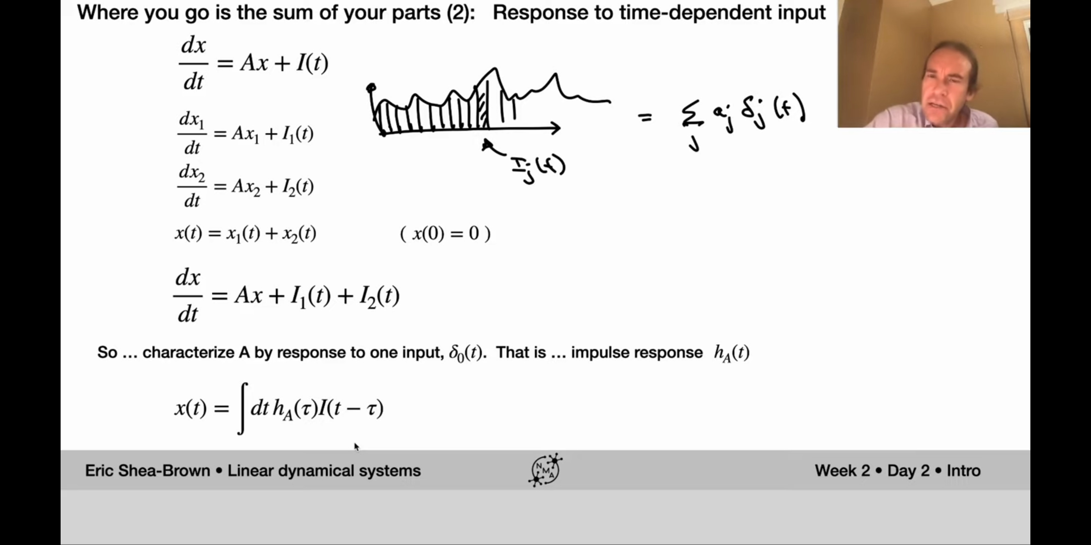
I’m not quite familiar with dynamical systems so these might be naive questions, but the derivation on this slide went over my head quite a bit:

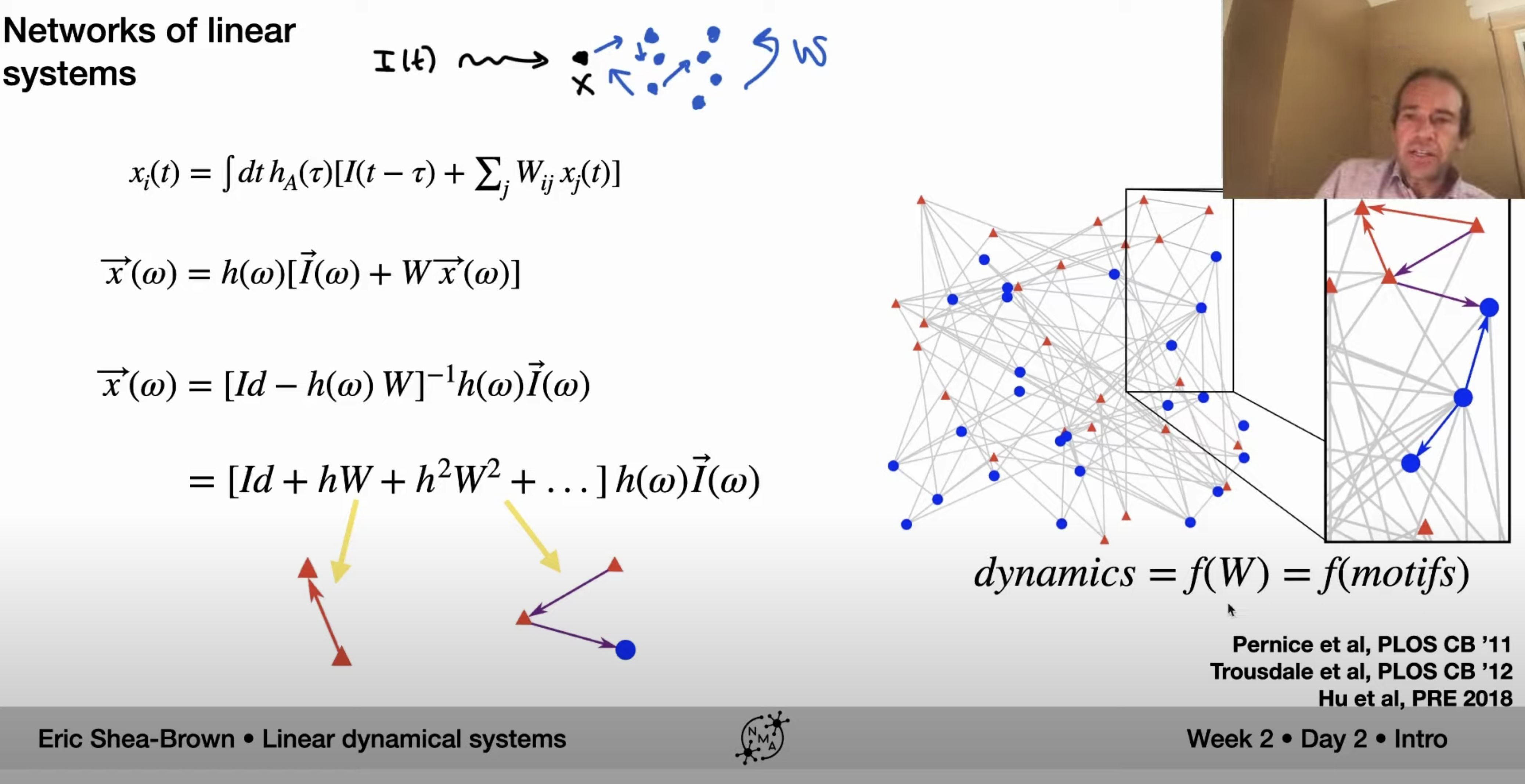
I’m wondering:

1. In general, could someone recommend good references for the analysis techniques introduced here?
2. Since we are stilling looking at a linear dynamical system (network), why we do introduce the frequency domain analysis, instead of keeping looking at eigenvalue/eigenvectors?
3. Could someone expand a bit more on the intuition of hW and h^2W^2 (and higher-order) terms here?

Thanks very much!

[ollimuh]

Need to do something of that sort (I believe…):

exp(-hW)= Id - hW + 1/2 h^2W^2 -...
–> need to subtract the squared term here, then, when doing the inversion it becomes additive (ignoring higher order terms)
and
exp(hW)= Id + hW + 1/2 h^2W^2 +...
… and this would give me the other half of the squared term.

[nalewkoz]

You can understand this by writing down the initial probability distribution as a linear combination of eigenvectors. The first one describes the equilibrium (stationary state). The second one describes the difference between the initial state and the equilibrium state (think about it as a ‘perturbation’). Since probabilities must add up to 1, perturbation in one component has to be counterbalanced by the perturbation in the other one. That’s why we get two components of exactly opposite signs. Note that what you see is a vector that is normalized in L2 norm.

[Maya_Wilde]

Ah, so it relates to the rate of the probabilities (in exercise 2b) moving towards the equilibrium, each by the same amount at each time step but in opposite directions?

[nalewkoz]

2. Frequency domain is extremely useful in applications, as looking at linear systems in the frequency (Fourier) domain simplifies the analysis (we can go from differential equations to algebraic equations). See also https://en.wikipedia.org/wiki/Normal_mode

3. This is a bit more fancy (we have matrices here, not scalars) geometric series (https://en.wikipedia.org/wiki/Geometric_series)

[11110]

Could anyone please elaborate on some things from Tutorial2, Section 1, State-change simulation process?

1. why do we need to scale c2o and o2c rates by dt?
2. why do we use random uniformly distributed numbers and compare them with scaled c2o and o2c rates, instead of directly using \mu_{c2o} and \mu_{o2c}

Part of code that seems to be confusing:

# Poisson processes

        if x[k] == 0 and myrand[k] < c2o*dt: # remember to scale by dt!

            x[k+1:] = 1

            switch_times.append(k*dt)

        elif x[k] == 1 and myrand[k] < o2c*dt:

            x[k+1:] = 0

            switch_times.append(k*dt)

[FedeClaudi]

The tutorials are so great for today! I was actually upset when I finished T4, I could’ve done 4 more

Agree that equilibria classification would’ve been a nice addition. Though I can imagine it has to be difficult to pack so much knowledge in a few hours worth of materials.

[likkkk]

After learning these tutorials, everything makes sense

[Adamreynolds28]

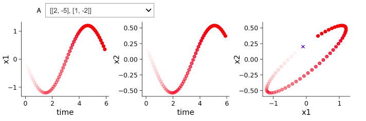
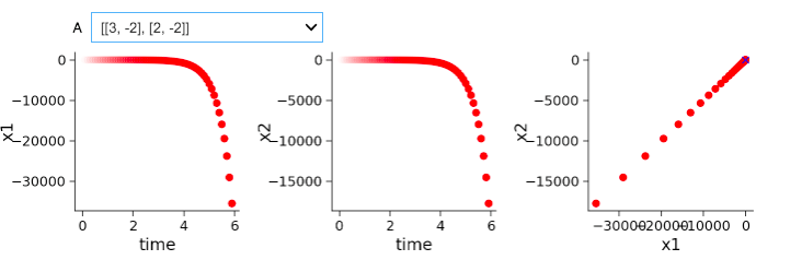
In T1 we were suppose to describe qualitatively how A influences the x1dot and x2dot system. It is not so intuitive the influence that negative and positive values have on the system. I am a bit confused.
In one set of negative and positive a values you have a decay and in another you have an oscillation. Is the difference purely due to a difference in magnitude?

[farbakhsh]

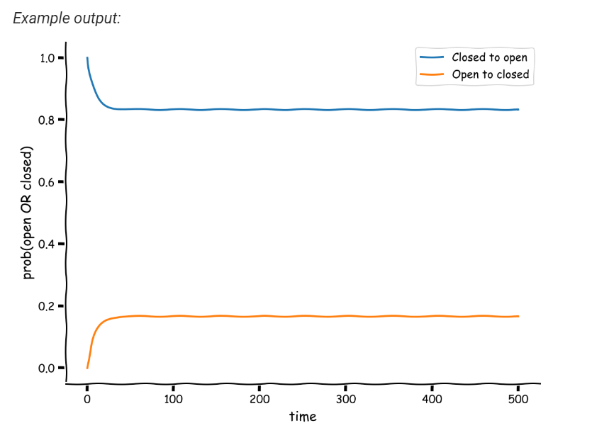
Are legends in this plot correct? Shouldn’t the blue one say “close” and the orange one “open”??

[NingMei]

For discrete time formulation, when the eigenvalues equal to 1, the eigenvectors are the stable solution. I guess this followed the tutorial slides page 38. But I still cannot intuitively understand how the case could be for continue time formulation.

[alex_ivanov]

Shouldn’t the integral here be over tau rather than t? This looks like the classic convolution equation.

[kevinwli]

This is probably wrong! see my second take below…

W2D2 - Content discussion

A second take on the second eigenvector… It is important to note that the eigen vectors are not orthonormal, so projection intuitions don’t really work. In short, v_2 is crucial in pulling state distributions towards stationarity. [image]

This might be an intuition. The second eigenvector satisfies:

(Ax).v_2 = \lambda_2 x.v_2, here \lambda_2<1

Dot product between x and v_2 is similar to taking the difference between the two probabilities, since v_2 \propto [-1,1]^\intercal

Since \lambda_2<1, this eigenvector has the effect of trying to reduce the difference between the two elements, making them go towards [0.5,0.5].

However, since v_2 is NOT orthogonal to v_1, v_1 also influences x with a larger eigenvalue.

[Haris_Organtzidis]

I do think so, yes. The integral is over tau and it is a convolution, which for me is easy to visualise if I think about it as a filter, as Eric does in the following seconds after the screenshot.

[NingMei]

[0.83333, 0.1666667] is not normalized. Am I wrong?

[decomite]

The sum of the elements is 1 but the vector is not of unit length indeed. If it has been normalized this is using L1 norm.

[Aakash]

Not sure if this question is asked before, Is it possible to determine that pattern of Eigen values (positive/negative) directly from the input matrix i.e. based on how the values change along each column. My guess is no but I would like to confirm it here.

Thanks
Aakash

[Haris_Organtzidis]

Kevin has written a nice explanation for our switching probabilities example below! More generally, I tried to give an intuition to the students by saying that what any matrix does when it gets multiplied by a vector is to rotate the vector and expand/contract it at the same time (and keep the vector in the same space if the matrix square). This happens to any x when we do Ax.

But the eigenproblem says that : Au = λu. In other words, if A gets multiplied by an eigenvector u, the resultant vector would be the same as if u would be multiplied by a scalar λ. So A does not rotate u, it only contracts/expands it (depending on λ). So as your x evolves, the closer it gets to a u direction, the less it changes in direction. When x has exactly the same direction as u, then it will stop changing direction at all and only contract/expand. So x in all future time step will be stuck on u’s direction, since there is no rotation (= no change in direction).

Note that Ax in the continuous case corresponds to x_dot, so the direction that your system changes in, will stop changing after x gets very close to an eigenvector direction. Your system will forever evolve on that direction from that point onwards, either to 0 or infinity (depending on λ).