In the interactive demo of tutorial 2 section 1, why does the widget specify dt to be 0.1? If it’s a discrete process, shouldn’t dt = 1? The result with dt = 0.1 is that when probabilities for c20 and o2c are both set to 1, the intervals aren’t always 0 (which they should be if ion channels are certain to switch immediately).
It looks indeed quite tricky. If the matrix is diagonal, the eigenvalues are the non-zeros values on the diagonal. If the matrix is not diagonal, you can make some guess about its eigenvalues but you need to have the derivation in mind which sounds tricky 
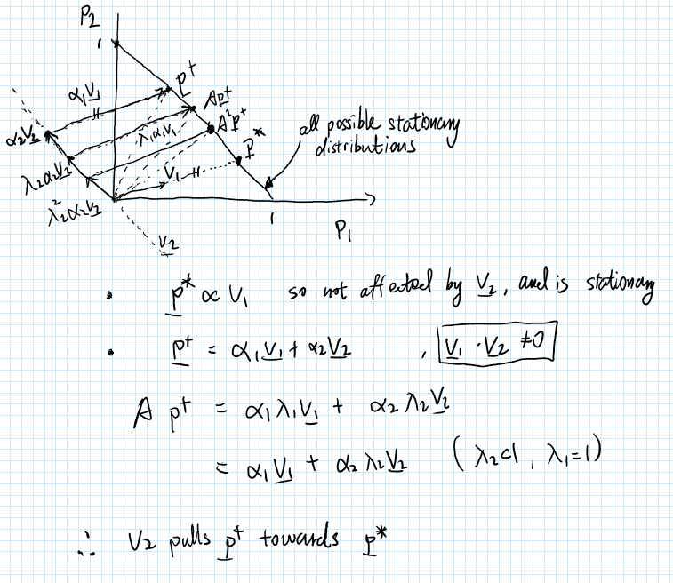
A second take on the second eigenvector…
It is important to note that the eigen vectors are not orthonormal, so intuitions based on orthogonal projection don’t really work.
In short, v_2 is the direction along which A pulls any p towards stationarity. \lambda_2 affects how fast or strong the pull is. A smaller \lambda_2 gives a faster convergence. According to a student in my pod @Daisy_duanqin77, \lambda_2 does not change the destiny, but only affects how fast destiny is fulfilled!
3 Likes
In the video for the first lecture, it is. said that all linear dynamical systems have this form:
x_dot = a*x
Which gives exp growth when a>0, exp decay when a<0 and no change if a=0.
However, I think it is possible to also have x_dot = a where there is no x term, which when integrated (solved) gives you just x = x_0 + a*t?
1 Like
Yeah, What I was trying to get at was without any derivation (i.e. in the matrix [[1 1 ][5 2]] the column whose values changes from 1 to 5 might have larger Eigen value than the column whose values change from 1 to 2). I don’t think that it is the case. Anyway, thanks for your help
There is a nice property that could help you identify how a modification of any entry of the matrix affects the eigenvalues.
The sum of eigenvalues multiplied by their algebraic multiplicity is equal to the trace of A while the determinant of A is equal to the product of its eigenvalues elevated by their algebraic multiplicity.
You then have a systems of 2 equations with 2 unknowns to solve which might provide better intuition that the characteristic polynomial.
A more straightforward/visual way to use the streamline plots (from T1) to display it, thats what i did during the tutorial. u just need to convert the disctrete transition matrix to continuous format: A_c = scipy.linalg.logm(A) / dt
1 Like
Due to the effect of each variable on the other one, it is usually not easy to use the entries of A directly (rather than its eigenvalues) to infer the behaviour of the system. In you top example, the eigenvalues are i and -i, so the system forms a stable cycle. In your second example, the eigenvalues are 2 and -1, so it’s a saddle (see also section 4 of the tutorial for the stream plots of these dynamics matrices)
2 Likes
I’m also very confused at this part. Can someone explain please?
It’s not normalized, unit vector. Since these two numbers represent probabilities, they should (and do) sum to zero.
1 Like
The rates c2o and o2c are in units of “probability per unit time.” Our simulation goes in units of dt, so at every dt, c2o and o2c need to be scaled down by multiplying by dt, otherwise the effective transition probabilities are way too big.
2 Likes
This is an excellent idea! Wish I had thought of it… 
1 Like
Can anyone explain why the variance of the OU process is 1/(lam^2) ? I’ve only ever seen this calculation of the variance (although to be honest, makes more sense to calculate covariance of x_t wrt another timepoint x_s)
Yeah, it’s a bit different in the discrete time formulation, which is the less common thing to derive than the continuous time formulation. The derivation is slightly involved, which is why I did not go through it in the lecture. I’m trying to dig up a website where someone has typed it up…
2 Likes
I also highly highly second the recommendation of Steve’s videos. I did my masters at UW which I’ve found prepared me excellently for comp. neuro. and these videos are essentially much of that degree but for free! J. Nathan Kutz also has some good ones on very related topics.
2 Likes
Wow, why is it that? Is there a quick ref to this property?
Did you mean why A_d = exp(A_c * dt)? For a continuous solution x_t = exp(A_c * t) * x_0, you have x_{k+1} = exp(A_c * (k+1) * dt) * x_0 = exp(A_c * dt) * exp(A_c * k * dt) * x_0 = exp(A_c * dt) * x_k.
1 Like
Ah I forgot about it being in discrete time, this makes sense thank you!!
I think you’re correct and that’s the convolution integral. that should be d(tau)