Hi there, recently I started to dive into the neural mass modelling. Things went pretty good until I faced The Virtual Brain and the model optimization based on the empirical data. TL; DR: some models don’t even oscillate with default values, and none provided a good resting state empirical FC fit, neither with optimal values found elsewhere nor with my own grid search optimization; I feel like I’m doing something terribly wrong, but I can’t figure this out.
First things first, I took the data from this dataset, specifically, I took the sub-009 participant. I preprocessed their anatomy with FreeSurfer’s recon-all with default parameters. I obtained the structural connectivity matrix from the DWI data by processing it with MRtrix, mainly following the Andy’s guide, except for the choice of the brain parcellation (I used “Schaefer100 + 56”, that is, Schaefer100 for 100 cortical regions assisted with 56 subcortical ones). Finally, I processed the fMRI data with fMRIprep followed by XCP-D; I used the default preprocessing pipeline in fMRIprep and the linc postprocessing mode in XCP-D. The last one was mostly unchanged except the file format that I switched from default cifti to nifti. Then I reformatted the structural connectivity matrix and the tract length matrix from csv to txt like this
def convert(file, output):
    data_dir = '/home/goliath/projects/datasets/trigeminal_neuralgia_dataset/derivatives_postproc/atlases/atlas-4S156Parcels'
    file_path = f'{data_dir}/{file}'
    output_path = f'{data_dir}/Conn/{output}'
    content = []
    with open(file_path) as f:
        content.extend(f.readlines())
    new_content = []
    for line in content:
        newline = line.replace(',', '\t')
        new_content.append(newline)
    with open(output_path, 'w') as f:
        f.writelines(new_content)

weights_file = 'sub-101_parcels_v3.csv'
weights_output = 'sub-101_weights.txt'
dist_file = 'sub-101_parcels_v3_length.csv'
dist_output = 'sub-101_tract_lengths.txt'
convert(weights_file, weights_output)
convert(dist_file, dist_output)
and place them in a dedicated folder that I named Conn. I also created a dummy coordinate centers file that is required by the TVB’s Connectivity.from_file method; I didn’t plan to simulate EEG/MEG, so I just set all these coordinates equal to zeros:
def extract_labels(file):
    parcel_info = []
    with open(f'{file}') as f:
        parcel_info.extend(f.readlines())
    labels = [el.split('\t')[1] for el in parcel_info]
    return labels[1:] # Header is omitted.

data_dir = '/home/goliath/projects/datasets/trigeminal_neuralgia_dataset/derivatives_postproc/atlases/atlas-4S156Parcels'
parcel_file = f'{data_dir}/atlas-4S156Parcels_dseg.tsv'
labels = extract_labels(parcel_file)
centre_file = f'{data_dir}/Conn/sub-101_centers.txt'
label_centres = []
for label in labels:
    label_centres.append(f'{label}\t0\t0\t0\n')
with open(centre_file, 'w') as f:
    f.writelines(label_centres)
This file was also placed in the Conn folder, which was then archived to a zip-file so that the TVB’s Connectivity.from_file method could use it. I started my journey with the Jansen-Rit model:
import numpy as np
from tvb.simulator.lab import models, connectivity, simulator, coupling, integrators, noise, monitors
import matplotlib.pyplot as plt

# Comment this to leave the default parameters, or don't.
nu_max=np.array([.005])
JR = models.JansenRit(nu_max=nu_max)

coup = coupling.SigmoidalJansenRit()

phi_n_scaling = (JR.a * JR.A * (JR.p_max-JR.p_min) * 0.5 )**2 / 2.
sigma         = np.zeros(6)
# Uncomment this to add noise.
# sigma[3]      = phi_n_scaling[0]

conn_dir = '/home/goliath/projects/datasets/trigeminal_neuralgia_dataset/derivatives_postproc/atlases/atlas-4S156Parcels'
conn = connectivity.Connectivity.from_file(f'{conn_dir}/Conn.zip')
# Uncomment this to simulate an isolated node.
# It's not a single isolated node per se, but with all conn weights down to zeros it becomes
# just a bunch of isolated nodes, so any can be chosen to explore the isolated node behaviour.
# conn.weights[:] = 0

sim = simulator.Simulator(
    model=JR,
    connectivity=conn,
    coupling=coup,
    integrator=integrators.HeunStochastic(dt=2 ** -4, noise=noise.Additive(nsig=sigma)),
    monitors=[monitors.Raw()],
    simulation_length=10e3,
).configure()

(time, data), = sim.run()

# All nodes.
plt.plot(time, data[:, 1, :, 0], 'k', alpha=0.1)
plt.show()
# One node.
plt.plot(time, data[:, 1, 154, 0], 'k', alpha=0.8)
plt.show()
# One node with transient skipped.
plt.plot(time[2000:], data[2000:, 1, 154, 0], 'k', alpha=0.8)
plt.show()
And this worked fine for an isolated node and, with some parameter tweaks, for the whole brain model, although I didn’t succeed in fitting the model to the empirical FC. Then I switched to the reduced Wong-Wang model with excitation and inhibition subpopulations, which is said to have 3 Hz oscilaltions for an isolated node (see article) with the default parameter values, but it does not oscillate at all nor it does with whatever parameter I tried. Here’s the code for the isolated node:
import numpy as np
from tvb.simulator.lab import models, connectivity, simulator, coupling, integrators, noise, monitors
import matplotlib.pyplot as plt

WW = models.ReducedWongWangExcInh()

coup = coupling.Linear(a=np.array([1]),b=np.array([0]))

sigma = 0.000 * np.ones((2, 156))

conn_dir = '/home/goliath/projects/datasets/trigeminal_neuralgia_dataset/derivatives_postproc/atlases/atlas-4S156Parcels'
conn = connectivity.Connectivity.from_file(f'{conn_dir}/Conn.zip')
# Single node.
conn.weights[:] = 0

sim = simulator.Simulator(
    model=WW,
    connectivity=conn,
    coupling=coup,
    integrator=integrators.HeunStochastic(dt=2 ** -4, noise=noise.Additive(nsig=sigma)),
    monitors=[monitors.Raw()],
    simulation_length=10e3,
).configure()

(time, data), = sim.run()

l = len(time)
s = np.round(0.6 * l).astype(int)
f = np.round(1 * l).astype(int)

plt.plot(time[s:f], data[s:f, 0, :, 0], 'k', alpha=0.1)
plt.show()
plt.plot(time[s:f], data[s:f, 0, 154, 0], 'k', alpha=0.8)
plt.show()
Finally, I tried Kuramoto model using as a reference this poster presentation. They use the same atlas that I do (Schaefer100) and they have the results of the parameter space exploration, so this is the closest study I could replicate without recalculating everything. I performed the grid search with two parameters, global connectivity strength and conduction speed:
import numpy as np
from tvb.simulator.lab import models, connectivity, simulator, coupling, integrators, noise, monitors
from tvb.analyzers.fmri_balloon import BalloonModel
from tvb.datatypes.time_series import TimeSeriesRegion
import matplotlib.pyplot as plt
import scipy as sp
import time as time_measure

N_a = 5
N_V = 5

corr_arr = np.zeros((N_a, N_V))

a_arr = np.linspace(73, 77, N_a)
V_arr = np.linspace(0.4, 0.6, N_V)
# If no parameter search is needed.
# a_arr = [75.]
# V_arr = [0.5]
for i_V, _V in enumerate(V_arr):
    for i_a, _a in enumerate(a_arr):
        start = time_measure.time()

        # The first 100 nodes are cortex, so here we are.
        N = 100

        omega = np.array([2 * np.pi * 60 / 1000])
        WW = models.Kuramoto(omega=omega)

        coup = coupling.Kuramoto(a=np.array([_a]))

        sigma = 0.000 * np.ones((1, N))

        conn_dir = '/home/goliath/projects/datasets/trigeminal_neuralgia_dataset/derivatives_postproc/atlases/atlas-4S156Parcels'
        conn = connectivity.Connectivity.from_file(f'{conn_dir}/Conn.zip')
        conn.speed = np.array([_V])
        conn.weights = conn.weights[0:N, 0:N]
        conn.tract_lengths = conn.tract_lengths[0:N, 0:N]
        conn.centres = conn.centres[0:N, 0:N]
        # conn.weights[:] = 0

        sim = simulator.Simulator(
            model=WW,
            connectivity=conn,
            coupling=coup,
            integrator=integrators.HeunStochastic(dt=2 ** -4, noise=noise.Additive(nsig=sigma)),
            monitors=[monitors.Bold()],
            simulation_length=60e3,

        ).configure()

        (time, data), = sim.run()

        # balloon = BalloonModel(time_series=TimeSeriesRegion(data=data, time=time))
        # bold = balloon.evaluate()

        sim_FC = np.zeros((N, N))
        for i in range(N):
            for j in range(N):
                sim_FC[i, j] = sp.stats.pearsonr(data[:, 0, i, 0], data[:, 0, j, 0])[0]
                # sim_FC[i, j] = sp.stats.pearsonr(bold.data[:, 0, i, 0], bold.data[:, 0, j, 0])[0]
        func_dir = '/home/goliath/projects/datasets/trigeminal_neuralgia_dataset/derivatives_postproc/sub-009/func'
        func_file = f'{func_dir}/sub-009_task-rest_space-MNI152NLin2009cAsym_seg-4S156Parcels_stat-pearsoncorrelation_relmat.tsv'
        func_content = []
        with open(func_file) as f:
            func_content.extend(f.readlines())

        emp_FC = np.zeros((N, N))
        for i, line in enumerate(func_content[:N+1]):
            if i == 0: continue
            values = np.array([float(el) if el != 'n/a' and el != 'n/a\n' else 0 for el in line.split('\t')[1:N+1]])
            emp_FC[i - 1, :] = values

        plt.imshow(emp_FC)
        plt.colorbar()
        plt.show()
        plt.imshow(sim_FC)
        plt.colorbar()
        plt.show()

        stop = time_measure.time()
        print('__________________________________________________')
        print(f'V is {_V}, corr is {sp.stats.pearsonr(emp_FC.flatten(), sim_FC.flatten())}')
        print(f'Elapsed time is {(stop - start) / 60}')
        print('__________________________________________________')

        corr_arr[i_a, i_V] = sp.stats.pearsonr(emp_FC.flatten(), sim_FC.flatten()).statistic
        l = len(time)
        s = np.round(0.0 * l).astype(int)
        f = np.round(1 * l).astype(int)

        plt.plot(time[s:f], data[s:f, 0, :, 0], 'k', alpha=0.1)
        plt.show()
        plt.plot(time[s:f], data[s:f, 0, N-1, 0], 'k', alpha=0.8)
        plt.show()

plt.imshow(corr_arr)
plt.xlabel('Conduction speed')
plt.gca().set_xticks(range(len(V_arr)), np.round(V_arr, 2))
plt.ylabel('Global coupling')
plt.gca().set_yticks(range(len(a_arr)), np.round(a_arr, 2))
plt.colorbar()
plt.show()
And still I achieved nothing. The optimal parameter values themselves, search in a small vicinity of them and search in broader borders, all of it resulted in no more than 0.1 correlation between the empirical and simulated FC, while 0.3-0.6 correlations were reported in studies I read.
So having said that, these are my questions:
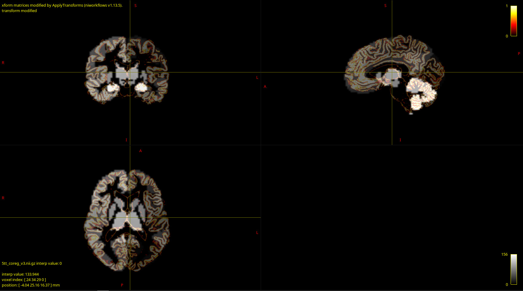
- How can I validate that my data is correct? After coregistration of parcellation image I overlaid it with anatomy and tractography images and they looked fine for me:
But I’m not experienced in that and, furthermore, MRtrix reported that one node in the structural connectome did not have tracts, which may indicate poor coregistration. If so, can the one node without tracts result in totally messed up fit? - My empirical FC and SC matrices seem to correlate weakly, just a bit more than 0.15. Is that OK or this is also a sign of bad input data?
- The Jansen-Rit model seems the most promising for me now, but what parameters of it should I use for the fitting process? In the literature, the global coupling strength is usually used, so should I use the c_max parameter of a coupling object (basically a coefficient before the coupling term), or, rather, J described as “Average number of synapses between populations”? Or another one?
- How can I force the Wong-Wang model to work? It’s so strange that it is widely used and still I can’t obtain any appropriate result from it, so I must be doing something wrong, but what exactly? Or do I totally misunderstand the model and it actually should not oscillate at all?
- While experimenting with Kuramoto model, I cropped the connectivity matrices to the first 100 nodes since they represent cortex. This did not result in improving the fit quality, but should I use carefully the parcellations with both cortical and subcortical regions? I feel like I should use different models for them, but should I really?
- I tried obtaining the simulated BOLD signal in two ways: with BOLD monitor and with Balloon model from TVB’s analyzers module. The solution for the Balloon model diverged for some reason so I could not use it, but what is the actual difference? Should I prefer one to another, at least, in case of the resting state?
- Finally, how do I perform the empirical FC fit at all? I could do some minor changes and search the optimal values thoroughly, but a long streak of fruitless simulations makes me think that I’m mistaken in some major point. What am I doing wrong?
- A little bit of an off-topic, if you please. I struggled a lot not only with the lack of results, but also with the way the TVB docs are written. For example, take a look at the models description. If you scan through the left-hand side panel, you’ll find the reduced Wong-Wang model (labeled “ReducedWongWang”). But if you actually need the reduced Wong-Wang with excitation and inhibition subpopulations, it’ll lead you astray since it is not the model you are looking for (even though it is called like this in studies). The model you actually need is ReducedWongWangExcInh, and it is simply not described here, although it is presented in the model enum and in the actual code base. So my question is not of technical matter, but rather I ask your opinion or a piece of advice: how do you think, is it worth to keep trying to master TVB, or is it better to switch to another library or even self-written code in something like Julia? Of course, this is not a question of the topic I created, so feel free to skip it if you want.

In addition to what I’ve written here I add a link to my Github repo where I place the code and the matrcies I used in my calculations, namely, SC, FC and tract length matrices, in case you need them. Thank you for your attention and help.